4种插值算法

如果有一些稀疏的轨迹，如何将这些轨迹平滑插值处理呢？

方法1：线性插值

方法2：三次样条插值

方法3：贝塞尔曲线插值

方法4：拉格朗日插值

线性插值：在两两相邻的点之间差值，两点间所有插值点都在一条直线上。

贝塞尔曲线：贝塞尔曲线不会经过所有的坐标点，会根据坐标点的排列趋势去拟合出一条相对平滑的从第1个点到最后一个点之间的曲线。

三次样条插值：插值函数会经过所有的坐标点，拟合函数平滑。

拉格朗日插值：点太多，会出现不稳定的结果。见下图：

前三种插值算法都有特定的使用场景，按需使用就好了。

import time

import numpy as np
from scipy.interpolate import interp1d
from scipy.special import comb


def linear_interpolation(route, num_points):
    # 1. 线性插值
    # 将经纬度分开
    lons = np.array([point[0] for point in route])
    lats = np.array([point[1] for point in route])

    # 创建插值函数
    distance = np.cumsum(np.sqrt(np.ediff1d(lons, to_begin=0) ** 2 + np.ediff1d(lats, to_begin=0) ** 2))
    distance /= distance[-1]

    # 创建插值函数
    lon_interp = interp1d(distance, lons, kind='linear')
    lat_interp = interp1d(distance, lats, kind='linear')

    # 生成新的距离点
    new_distance = np.linspace(0, 1, num_points)

    # 插值
    new_lons = lon_interp(new_distance)
    new_lats = lat_interp(new_distance)

    return list(zip(new_lons, new_lats))


def cubic_spline_interpolation(route, num_points):
    # 2. 三次样条插值
    lons = np.array([point[0] for point in route])
    lats = np.array([point[1] for point in route])

    distance = np.cumsum(np.sqrt(np.ediff1d(lons, to_begin=0) ** 2 + np.ediff1d(lats, to_begin=0) ** 2))
    distance /= distance[-1]

    lon_interp = interp1d(distance, lons, kind='cubic')
    lat_interp = interp1d(distance, lats, kind='cubic')

    new_distance = np.linspace(0, 1, num_points)

    new_lons = lon_interp(new_distance)
    new_lats = lat_interp(new_distance)

    return list(zip(new_lons, new_lats))


def bernstein_poly(i, n, t):
    return comb(n, i) * (t ** i) * ((1 - t) ** (n - i))


def bezier_curve(route, num_points=100):
    # 3. 贝塞尔曲线插值
    n = len(route) - 1
    t = np.linspace(0, 1, num_points)

    lons = np.array([point[0] for point in route])
    lats = np.array([point[1] for point in route])

    new_lons = np.zeros(num_points)
    new_lats = np.zeros(num_points)

    for i in range(n + 1):
        new_lons += bernstein_poly(i, n, t) * lons[i]
        new_lats += bernstein_poly(i, n, t) * lats[i]

    return list(zip(new_lons, new_lats))


import matplotlib.pyplot as plt


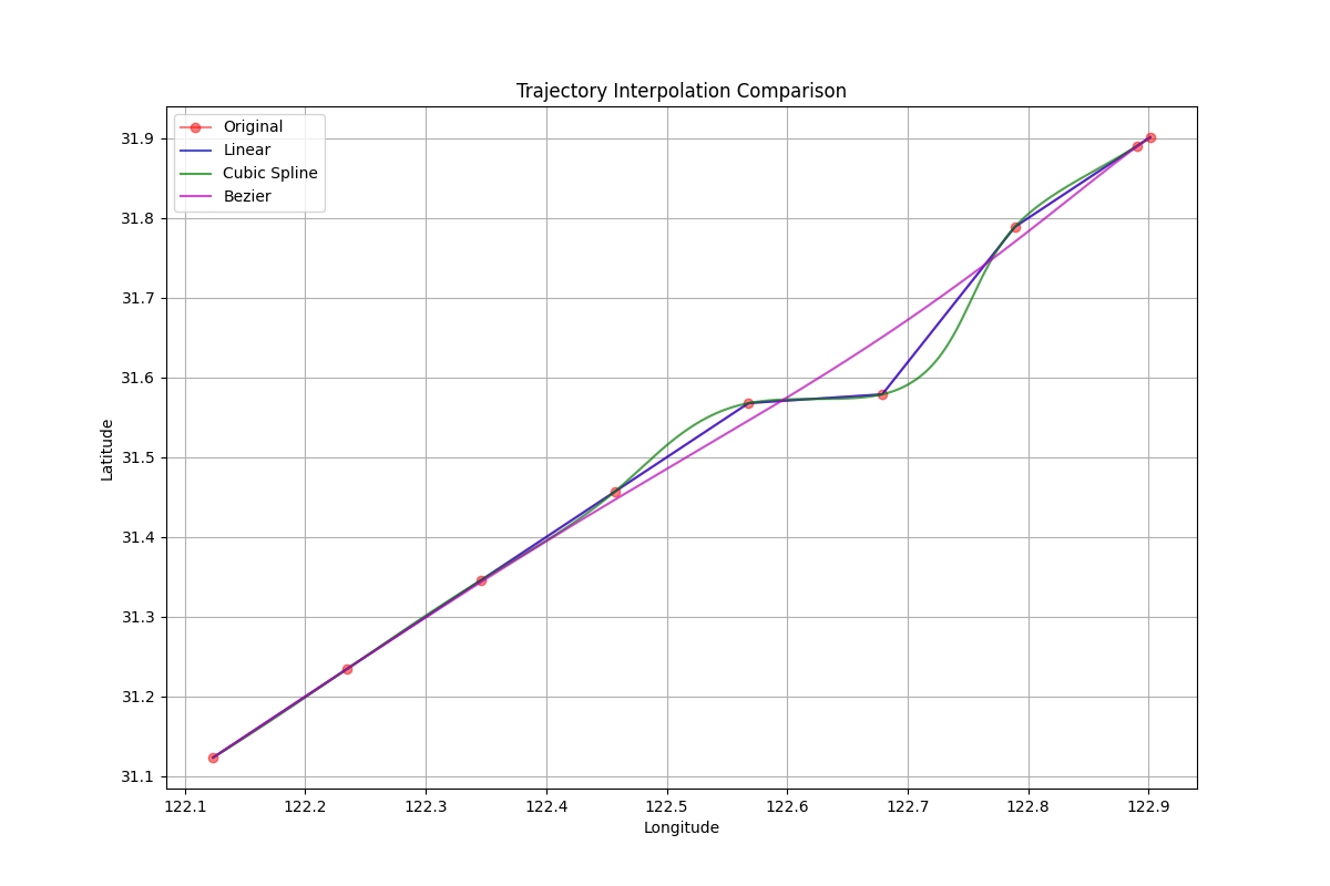
def plot_routes(original, linear, cubic, bezier):
    plt.figure(figsize=(12, 8))

    # 原始轨迹
    orig_lons, orig_lats = zip(*original)
    plt.plot(orig_lons, orig_lats, 'ro-', label='Original', alpha=0.5)

    # 线性插值
    lin_lons, lin_lats = zip(*linear)
    plt.plot(lin_lons, lin_lats, 'b-', label='Linear', alpha=0.7)

    # 三次样条插值
    cub_lons, cub_lats = zip(*cubic)
    plt.plot(cub_lons, cub_lats, 'g-', label='Cubic Spline', alpha=0.7)

    # 贝塞尔曲线
    bez_lons, bez_lats = zip(*bezier)
    plt.plot(bez_lons, bez_lats, 'm-', label='Bezier', alpha=0.7)

    plt.legend()
    plt.xlabel('Longitude')
    plt.ylabel('Latitude')
    plt.title('Trajectory Interpolation Comparison')
    plt.grid(True)
    plt.show()


if __name__ == '__main__':
    # 原始轨迹数据
    route = [
        [122.123456, 31.123456],
        [122.234567, 31.234567],
        [122.345678, 31.345678],
        [122.456789, 31.456789],
        [122.567890, 31.567890],
        [122.678901, 31.578901],
        [122.789012, 31.789012],
        [122.890123, 31.890123],
        [122.901234, 31.901234],
    ]
    start_time = time.time()
    # 线性插值
    linear_route = linear_interpolation(route, 1000)
    print("线性插值结果 (前5个点):", linear_route[:5])
    print("线性插值用时:", time.time() - start_time, "秒")

    start_time = time.time()
    # 三次样条插值
    cubic_route = cubic_spline_interpolation(route, 1000)
    print("三次样条插值结果 (前5个点):", cubic_route[:5])
    print("三次样条插值用时:", time.time() - start_time, "秒")

    start_time = time.time()
    # 贝塞尔曲线插值
    bezier_route = bezier_curve(route, 1000)
    print("贝塞尔曲线插值结果 (前5个点):", bezier_route[:5])
    print("贝塞尔曲线插值用时:", time.time() - start_time, "秒")

    # 绘制比较图
    plot_routes(route, linear_route, cubic_route, bezier_route)

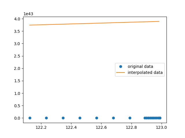
# 4、拉格朗日插值算法
import time

from scipy.interpolate import lagrange
import numpy as np


def lagrange_interp(x, y, x_new):
    """
    Lagrange interpolation
    :param x: x coordinates of data points
    :param y: y coordinates of data points
    :param x_new: x coordinates of new interpolated points
    :return: y coordinates of new interpolated points
    """
    f = lagrange(x, y)
    y_new = f(x_new)
    return y_new


if __name__ == '__main__':
    # 原始数据
    route = [
        [122.123456, 31.123456],
        [122.234567, 31.234567],
        [122.345678, 31.345678],
        [122.456789, 31.456789],
        [122.567890, 31.567890],
        [122.678901, 31.678901],
        [122.789012, 31.789012],
        [122.890123, 31.890123],
        [122.901234, 31.901234],

    ]

    x_list = [i[0] for i in route]
    y_list = [i[1] for i in route]
    # 新数据
    x_new = np.arange(122.123456, 122.990123, 0.01)
    y_new = lagrange_interp(x_list, y_list, x_new)
    # 绘图
    import matplotlib.pyplot as plt

    plt.plot(x_list, y_list, 'o', label='original data')
    plt.plot(x_new, y_new, label='interpolated data')
    plt.legend()
    plt.show()