引言
前序学习进程中,已经学习了超平面的基础知识,学习链接为:超平面
在此基础上,要想正确绘制超平面,还需要了解感知机的相关概念。
感知机
感知机是对生物神经网络的模拟,当输入信号达到感知机的阈值时,会输出感应信号,否则不会有任何反应。
这里先对感知机建立数学模型。
对于向量F和向量G,有:
F ˉ = ( f 0 , f 1 , f 2 , . . . , f n ) , G ˉ = ( g 0 , g 1 , g 2 , . . . , g n ) \bar {F}=(f0,f1,f2,...,fn),\bar{G}=(g0,g1,g2,...,gn) Fˉ=(f0,f1,f2,...,fn),Gˉ=(g0,g1,g2,...,gn)定义向量点积: H = F ˉ ⋅ G ˉ \ H=\bar {F} \cdot \bar {G} H=Fˉ⋅Gˉ
如果满足:
H = { 1 if H ≥ 0 − 1 if H < 0 H=\left\{ \begin{matrix} 1 \quad \text{\quad if } H\geq 0 \\ -1 \quad \text{if } H< 0 \end{matrix} \right. H={1if H≥0−1if H<0
相应的,在numpy模块中,也有一个sign()函数可以对感知机的数学模型进行精炼表达,这有一个代码实例:
python
# 引入numpy模块
import numpy as np
# 引入数据
x=[1,2,3,-6,-8,-10]
# np.sign()函数测试
z=np.sign(x)
print('z=',z)
代码运行后的输出效果为:
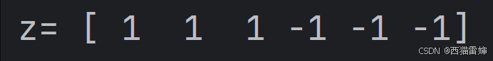
非常明显,对于非负数,np.sign()函数输出1,对于负数则直接输出0。
一个关于感知机的项目
这里有一个感知机算法的简单项目:
python
# 引入模块
import numpy as np
import matplotlib.pyplot as plt
from sklearn.datasets import make_classification
from matplotlib.colors import ListedColormap

# 定义随机数种子
# 定义了随机数种子后,每次产生的随机数是一样的
# 使用不同的随机数种子,会得到不同的初始随机数
np.random.seed(88)

def perceptron_learning_algorithm(x, y):
    # W是3个在[0,1)区间上均匀分布的随机数
    w = np.random.rand(3)
    # misclassified_examples是由predict()函数计算获得
    misclassified_examples = predict(hypothesis, x, y, w)

    while misclassified_examples.any():
        x_example, expect_y = pick_one_from(misclassified_examples, x, y)
        # 更新权重
        w = w + x_example * expect_y
        # 重新代入predict()函数进行评估
        misclassified_examples = predict(hypothesis, x, y, w)
    return w

# hypothesis函数对w和x两个向量的点积进行感知机运算
# hypothesis函数返回值是1或者-1
def hypothesis(x, w):
    return np.sign(np.dot(w, x))

# predict函数包括4个变量
def predict(hypothesis_function, x, y, w):
    # np.apply_along_axis函数先将x按照行取出,这是由axis=1决定的取值方式
    # hypothesis_function每次接收x的一行和w
    predictions = np.apply_along_axis(hypothesis_function, 1, x, w)
    # y != predictions表示分类错误,这个!代表的不等于判断会输出布尔结果False和True
    # x[y != predictions]直接输出x[y != predictions]取值为True时对应x行的数据
    misclassified = x[y != predictions]
    return misclassified

# pick_one_from函数
def pick_one_from(misclassified_examples, x, y):
    # 随机打乱分类样本的顺序
    np.random.shuffle(misclassified_examples)
    t = misclassified_examples[0]
    index = np.where(np.all(x == t, axis=1))[0][0]
    return x[index], y[index]

# 使用sklearn生成线性可分的数据集
x, y = make_classification(
    n_samples=100,
    n_features=2,
    n_redundant=0,
    n_informative=2,
    n_clusters_per_class=1,
    random_state=42,
    class_sep=2.0
)

# 将标签从0/1转换为-1/1
y = np.where(y == 0, -1, 1)

# 添加偏置项
x_augmented = np.c_[np.ones(x.shape[0]), x]

# 训练感知机模型
w = perceptron_learning_algorithm(x_augmented, y)
print("感知机权重:", w)

# 绘制分类效果图
plt.figure(figsize=(10, 8))

# 绘制数据点
plt.scatter(x[y==1][:, 0], x[y==1][:, 1], c='blue', marker='o', label='Class +1', edgecolor='k', s=70)
plt.scatter(x[y==-1][:, 0], x[y==-1][:, 1], c='red', marker='o', label='Class -1', s=70)

# 绘制决策边界
x_min, x_max = x[:, 0].min() - 1, x[:, 0].max() + 1
y_min, y_max = x[:, 1].min() - 1, x[:, 1].max() + 1

xx, yy = np.meshgrid(np.arange(x_min, x_max, 0.02),
                     np.arange(y_min, y_max, 0.02))

# 预测网格点的分类
Z = np.array([hypothesis(np.array([1, a, b]), w) for a, b in zip(xx.ravel(), yy.ravel())])
Z = Z.reshape(xx.shape)

# 绘制分类区域
cmap_light = ListedColormap(['#FFAAAA', '#AAAAFF'])
plt.contourf(xx, yy, Z, cmap=cmap_light, alpha=0.3)

# 绘制决策边界
plt.contour(xx, yy, Z, levels=[0], linewidths=2, colors='black')

# 添加图例和标题
plt.title('Perceptron Classification Results', fontsize=16)
plt.xlabel('Feature 1', fontsize=14)
plt.ylabel('Feature 2', fontsize=14)
plt.legend(loc='upper right', fontsize=12)
plt.grid(True, linestyle='--', alpha=0.7)
plt.tight_layout()

plt.show()
代码运行后,会获得直接的分类效果:
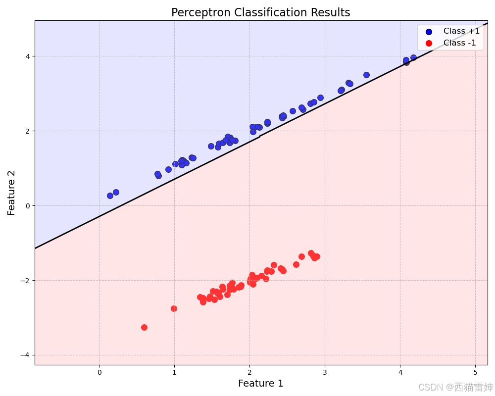
下一件文章将详细解读代码。
总结
学习了感知机的基本概念。