【数据分析】03 - pandas
文章目录
- [【数据分析】03 - pandas](#【数据分析】03 - pandas)
一:Pandas入门
1:Pandas概述
Pandas 一个强大的分析结构化数据的工具集,基础是 numpy
Pandas 官网 https://pandas.pydata.org/
Pandas 源代码:https://github.com/pandas-dev/pandas
- Pandas 可以从各种文件格式比如 CSV、JSON、SQL、Microsoft Excel 导入数据。
- Pandas 可以对各种数据进行运算操作,比如归并、再成形、选择,还有数据清洗和数据加工特征。
- Pandas 广泛应用在学术、金融、统计学等各个数据分析领域。
Pandas 是数据分析的利器,它不仅提供了高效、灵活的数据结构,还能帮助你以极低的成本完成复杂的数据操作和分析任务。
Pandas 提供了丰富的功能,包括:
- 数据清洗:处理缺失数据、重复数据等。
- 数据转换:改变数据的形状、结构或格式。
- 数据分析:进行统计分析、聚合、分组等。
- 数据可视化:通过整合 Matplotlib 和 Seaborn 等库,可以进行数据可视化。
shell
# 安装pandas
pip install pandas
python
# 测试pandas的安装
import pandas as pd

def pandas_test01():
    print(pd.__version__)


if __name__ == '__main__':
    pandas_test01()
pandas的特点如下
高效的数据结构:
- Series:一维数据结构,类似于列表(List),但拥有更强的功能,支持索引。
- DataFrame:二维数据结构,类似于表格或数据库中的数据表,行和列都具有标签(索引)。
数据清洗与预处理:
- Pandas 提供了丰富的函数来处理缺失值、重复数据、数据类型转换、字符串操作等,帮助用户轻松清理和转换数据。
数据操作与分析:
- 支持高效的数据选择、筛选、切片,按条件提取数据、合并、连接多个数据集、数据分组、汇总统计等操作。
- 可以进行复杂的数据变换,如数据透视表、交叉表、时间序列分析等。
数据读取与导出:
- 支持从各种格式的数据源读取数据,如 CSV、Excel、JSON、SQL 数据库等。
- 也可以将处理后的数据导出为不同格式,如 CSV、Excel 等。
数据可视化:
- 通过与 Matplotlib 和其他可视化工具的集成,Pandas 可以快速生成折线图、柱状图、散点图等常见图表。
时间序列分析:
- 支持强大的时间序列处理功能,包括日期的解析、重采样、时区转换等。
性能与优化:
- Pandas 优化了大规模数据处理,提供高效的向量化操作,避免了使用 Python 循环处理数据的低效。
- 还支持一些内存优化技术,比如使用
category类型处理重复的数据。
2:Pands数据结构
Series + DataFrame

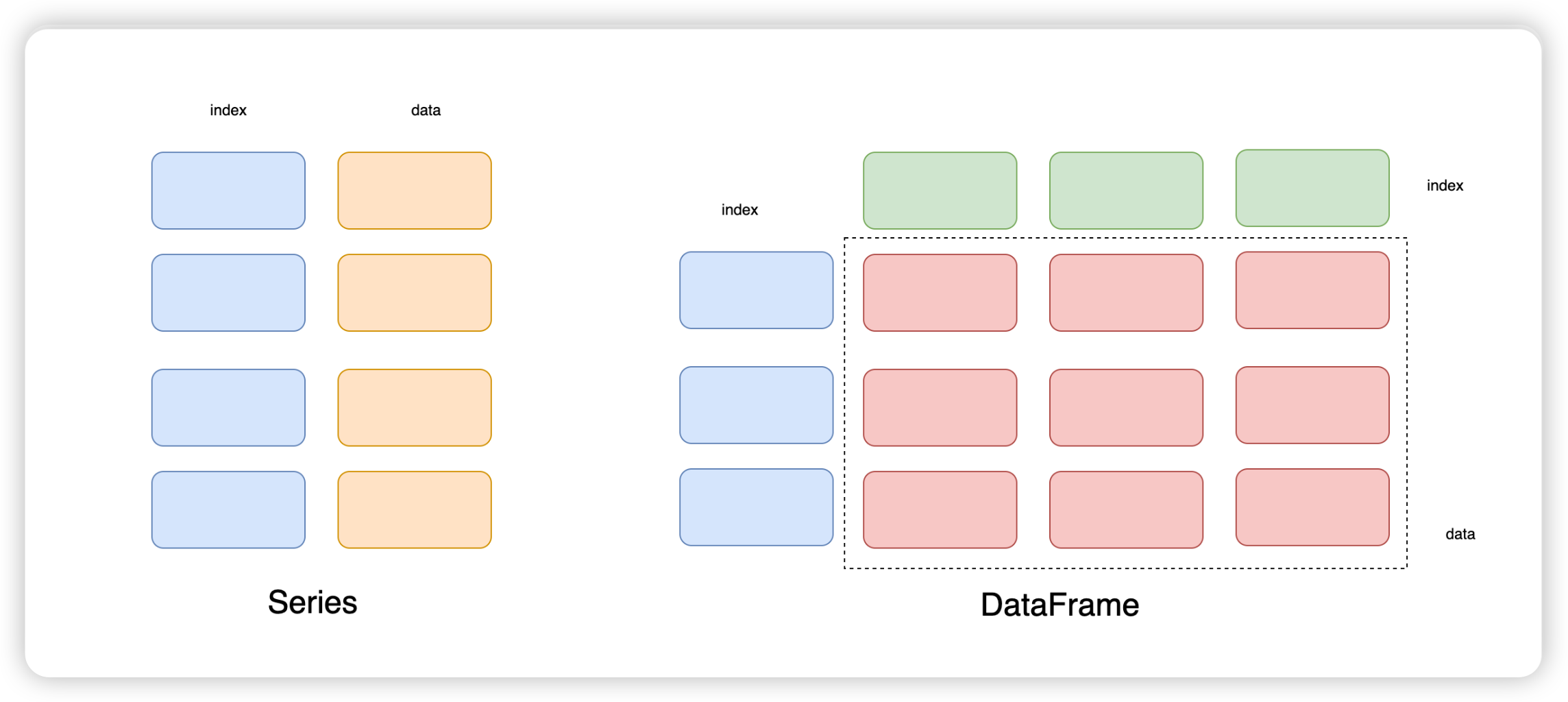
DataFrame 可视为由多个 Series 组成的数据结构:
- index是自动生成的,表示记录1 ~ 记录n
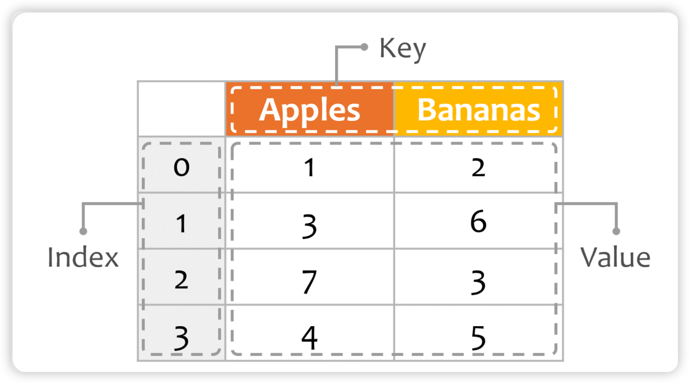
- 每一列表示一个Series, 列的名称就是key
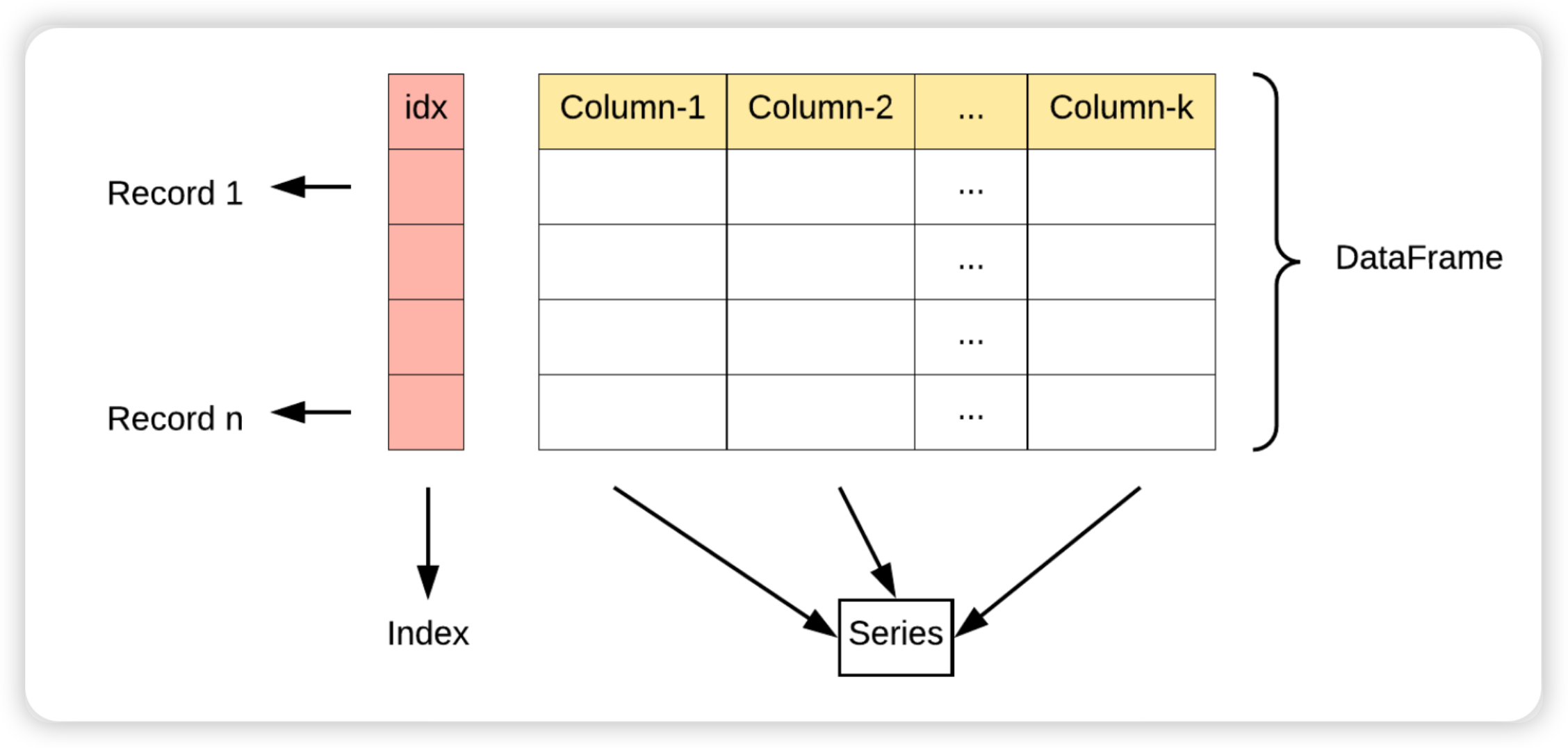
DataFrame = key + value + index
python
import pandas as pd
def pandas_test01():
print(pd.__version__)
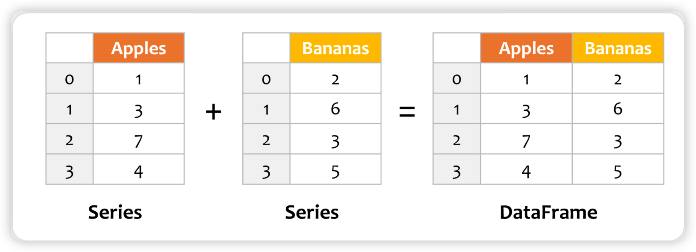
def pandas_test02():
# 创建两个Series对象
series_apples = pd.Series([1, 3, 7, 4])
series_bananas = pd.Series([2, 6, 3, 5])
# 将两个Series对象相加,得到DataFrame,并指定列名
df = pd.DataFrame({'Apples': series_apples, 'Bananas': series_bananas})
# 显示DataFrame
print(df)
if __name__ == '__main__':
pandas_test02()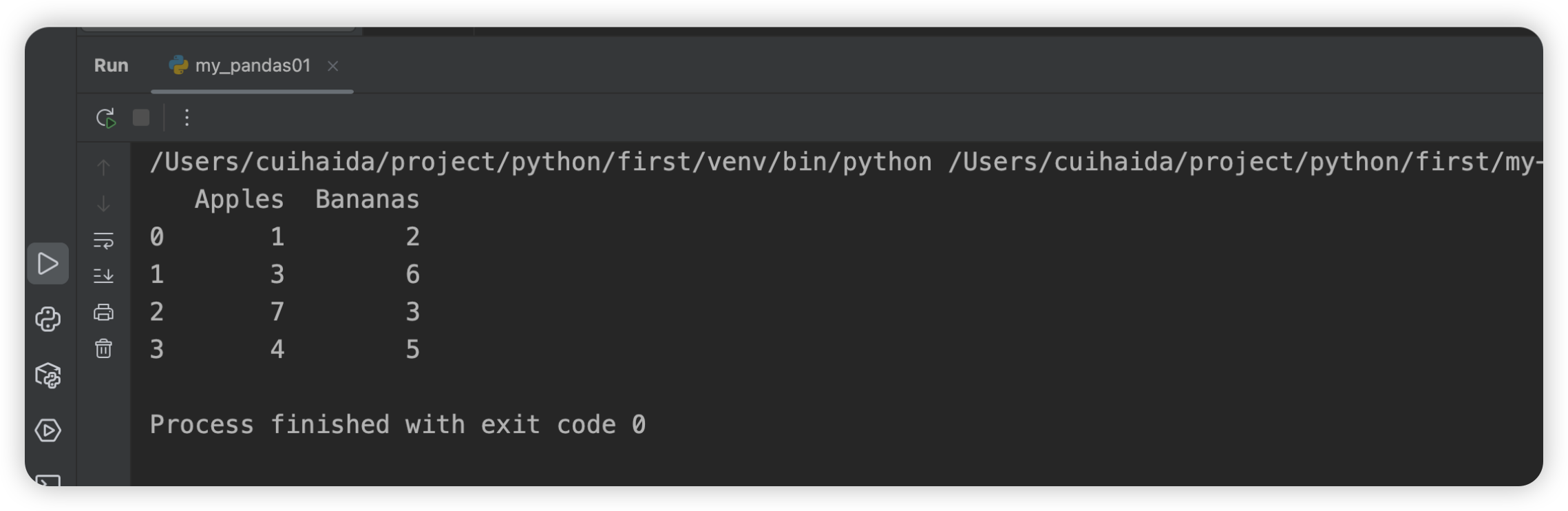
二:输入格式详解
1:CSV
CSV 是一种通用的、相对简单的文件格式,被用户、商业和科学广泛应用。
1.1:基本使用
pandas和CSV之间就是两个方法:
- 从CSV中读取数据,并加载成为DataFrame ->
pd.read_csv() - 将DataFrame中的内容写入到CSV ->
DataFrame.to_csv()
read_csv 常用参数:
| 参数 | 说明 | 默认值 |
|---|---|---|
filepath_or_buffer |
CSV 文件的路径或文件对象(支持 URL、文件路径、文件对象等) | 必需参数 |
sep |
定义字段分隔符,默认是逗号(,),可以改为其他字符,如制表符(\t) |
',' |
header |
指定行号作为列标题,默认为 0(表示第一行),或者设置为 None 没有标题 |
0 |
names |
自定义列名,传入列名列表 | None |
index_col |
用作行索引的列的列号或列名 | None |
usecols |
读取指定的列,可以是列的名称或列的索引 | None |
dtype |
强制将列转换为指定的数据类型 | None |
skiprows |
跳过文件开头的指定行数,或者传入一个行号的列表 | None |
nrows |
读取前 N 行数据 | None |
na_values |
指定哪些值应视为缺失值(NaN) | None |
skipfooter |
跳过文件结尾的指定行数 | 0 |
encoding |
文件的编码格式(如 utf-8,latin1 等) |
None |
to_csv 常用参数:
| 参数 | 说明 | 默认值 |
|---|---|---|
path_or_buffer |
CSV 文件的路径或文件对象(支持文件路径、文件对象) | 必需参数 |
sep |
定义字段分隔符,默认是逗号(,),可以改为其他字符,如制表符(\t) |
',' |
index |
是否写入行索引,默认 True 表示写入索引 |
True |
columns |
指定写入的列,可以是列的名称列表 | None |
header |
是否写入列名,默认 True 表示写入列名,设置为 False 表示不写列名 |
True |
mode |
写入文件的模式,默认是 w(写模式),可以设置为 a(追加模式) |
'w' |
encoding |
文件的编码格式,如 utf-8,latin1 等 |
None |
line_terminator |
定义行结束符,默认为 \n |
None |
quoting |
设置如何对文件中的数据进行引号处理(0-3,具体引用方式可查文档) | None |
quotechar |
设置用于引用的字符,默认为双引号 " |
'"' |
date_format |
自定义日期格式,如果列包含日期数据,则可以使用此参数指定日期格式 | None |
doublequote |
如果为 True,则在写入时会将包含引号的文本使用双引号括起来 |
True |
python
import pandas as pd

# 读取 CSV 文件,并自定义列名和分隔符
df = pd.read_csv('data.csv', sep=';', header=0, names=['A', 'B', 'C'], dtype={'A': int, 'B': float})
print(df)

# 假设 df 是一个已有的 DataFrame
df.to_csv('output.csv', index=False, header=True, columns=['A', 'B'])
1.2:数据处理
2:Excel
| 操作 | 方法 | 说明 |
|---|---|---|
| 读取 Excel 文件 | pd.read_excel() |
读取 Excel 文件,返回 DataFrame |
| 将 DataFrame 写入 Excel | DataFrame.to_excel() |
将 DataFrame 写入 Excel 文件 |
| 加载 Excel 文件 | pd.ExcelFile() |
加载 Excel 文件并访问多个表单 |
| 使用 ExcelWriter 写多个表单 | pd.ExcelWriter() |
写入多个 DataFrame 到同一 Excel 文件的不同表单 |
2.1:读取文件
读取excel方法的参数说明
| 参数 | 描述 |
|---|---|
io |
这是必需的参数,指定了要读取的 Excel 文件的路径或文件对象。 |
sheet_name=0 |
指定要读取的工作表名称或索引。默认为0,即第一个工作表。 |
header=0 |
指定用作列名的行。默认为0,即第一行。 |
names=None |
用于指定列名的列表。如果提供,将覆盖文件中的列名。 |
index_col=None |
指定用作行索引的列。可以是列的名称或数字。 |
usecols=None |
指定要读取的列。可以是列名的列表或列索引的列表。 |
dtype=None |
指定列的数据类型。可以是字典格式,键为列名,值为数据类型。 |
engine=None |
指定解析引擎。默认为None,pandas 会自动选择。 |
converters=None |
用于转换数据的函数字典。 |
true_values=None |
指定应该被视为布尔值True的值。 |
false_values=None |
指定应该被视为布尔值False的值。 |
skiprows=None |
指定要跳过的行数或要跳过的行的列表。 |
nrows=None |
指定要读取的行数。 |
na_values=None |
指定应该被视为缺失值的值。 |
keep_default_na=True |
指定是否要将默认的缺失值(例如NaN)解析为NA。 |
na_filter=True |
指定是否要将数据转换为NA。 |
verbose=False |
指定是否要输出详细的进度信息。 |
parse_dates=False |
指定是否要解析日期。 |
date_parser=<no_default> |
用于解析日期的函数。 |
date_format=None |
指定日期的格式。 |
thousands=None |
指定千位分隔符。 |
decimal='.' |
指定小数点字符。 |
comment=None |
指定注释字符。 |
skipfooter=0 |
指定要跳过的文件末尾的行数。 |
storage_options=None |
用于云存储的参数字典。 |
dtype_backend=<no_default> |
指定数据类型后端。 |
engine_kwargs=None |
传递给引擎的额外参数字典。 |
python
import pandas as pd

# 读取默认的第一个表单
df = pd.read_excel('data.xlsx')
print(df)

# 读取指定表单的内容(表单名称)
df = pd.read_excel('data.xlsx', sheet_name='Sheet1')
print(df)

# 读取多个表单,返回一个字典
dfs = pd.read_excel('data.xlsx', sheet_name=['Sheet1', 'Sheet2'])
print(dfs)

# 自定义列名并跳过前两行
df = pd.read_excel('data.xlsx', header=None, names=['A', 'B', 'C'], skiprows=2)
print(df)
2.2:写入文件
to_excel()方法的参数说明
| 参数 | 描述 |
|---|---|
excel_writer |
这是必需的参数,指定了要写入的 Excel 文件路径或文件对象。 |
sheet_name='Sheet1' |
指定写入的工作表名称,默认为 'Sheet1'。 |
na_rep='' |
指定在 Excel 文件中表示缺失值(NaN)的字符串,默认为空字符串。 |
float_format=None |
指定浮点数的格式。如果为 None,则使用 Excel 的默认格式。 |
columns=None |
指定要写入的列。如果为 None,则写入所有列。 |
header=True |
指定是否写入列名作为第一行。如果为 False,则不写入列名。 |
index=True |
指定是否写入索引作为第一列。如果为 False,则不写入索引。 |
index_label=None |
指定索引列的标签。如果为 None,则不写入索引标签。 |
startrow=0 |
指定开始写入的行号,默认从第0行开始。 |
startcol=0 |
指定开始写入的列号,默认从第0列开始。 |
engine=None |
指定写入 Excel 文件时使用的引擎,默认为 None,pandas 会自动选择。 |
merge_cells=True |
指定是否合并单元格。如果为 True,则合并具有相同值的单元格。 |
inf_rep='inf' |
指定在 Excel 文件中表示无穷大值的字符串,默认为 'inf'。 |
freeze_panes=None |
指定冻结窗格的位置。如果为 None,则不冻结窗格。 |
storage_options=None |
用于云存储的参数字典。 |
engine_kwargs=None |
传递给引擎的额外参数字典。 |
python
import pandas as pd

# 创建一个简单的 DataFrame
df = pd.DataFrame({
'Name': ['Alice', 'Bob', 'Charlie'],  # 第一列
'Age': [25, 30, 35], # 第二列
'City': ['New York', 'Los Angeles', 'Chicago'] # 第三列
})

# 将 DataFrame 写入 Excel 文件,写入 'Sheet1' 表单
df.to_excel('output.xlsx', sheet_name='Sheet1', index=False)

# 写入多个表单,使用 ExcelWriter
with pd.ExcelWriter('output2.xlsx') as writer:
    df.to_excel(writer, sheet_name='Sheet1', index=False)
    df.to_excel(writer, sheet_name='Sheet2', index=False)
2.3:加载文件
ExcelFile - 加载 Excel 文件
python
import pandas as pd

# 使用 ExcelFile 加载 Excel 文件
excel_file = pd.ExcelFile('data.xlsx')

# 查看所有表单的名称
print(excel_file.sheet_names)

# 读取指定的表单
df = excel_file.parse('Sheet1')
print(df)

# 关闭文件
excel_file.close()
2.4:多个表单的写入
可以使用ExcelWriter写入df到指定excel的指定sheet中
python
df1 = pd.DataFrame([["AAA", "BBB"]], columns=["Spam", "Egg"])
df2 = pd.DataFrame([["ABC", "XYZ"]], columns=["Foo", "Bar"])
with pd.ExcelWriter("path_to_file.xlsx") as writer:
    df1.to_excel(writer, sheet_name="Sheet1")
    df2.to_excel(writer, sheet_name="Sheet2")
3:JSON
| 操作 | 方法 | 说明 |
|---|---|---|
| 从 JSON 文件/字符串读取数据 | pd.read_json() |
从 JSON 数据中读取并加载为 DataFrame |
| 将 DataFrame 转换为 JSON | DataFrame.to_json() |
将 DataFrame 转换为 JSON 格式的数据,可以指定结构化方式 |
| 支持 JSON 结构化方式 | orient 参数 |
支持多种结构化方式,如 split、records、columns |
3.1:读取Json文件
python
import pandas as pd

df = pd.read_json(
    path_or_buffer,      # JSON 文件路径、JSON 字符串或 URL
    orient=None,         # JSON 数据的结构方式,默认是 'columns'
    dtype=None,          # 强制指定列的数据类型
    convert_axes=True,   # 是否转换行列索引
    convert_dates=True,  # 是否将日期解析为日期类型
    keep_default_na=True # 是否保留默认的缺失值标记
)| rient 值 | JSON 格式示例 | 描述 |
|---|---|---|
split |
{"index":["a","b"],"columns":["A","B"],"data":[[1,2],[3,4]]} |
使用键 index、columns 和 data 结构 |
records |
[{"A":1,"B":2},{"A":3,"B":4}] |
每个记录是一个字典,表示一行数据 |
index |
{"a":{"A":1,"B":2},"b":{"A":3,"B":4}} |
使用索引为键,值为字典的方式 |
columns |
{"A":{"a":1,"b":3},"B":{"a":2,"b":4}} |
使用列名为键,值为字典的方式 |
values |
[[1,2],[3,4]] |
只返回数据,不包括索引和列名 |
3.2:DF读取为JSON
python
df.to_json(
    path_or_buffer=None,    # 输出的文件路径或文件对象,如果是 None 则返回 JSON 字符串
    orient=None,            # JSON 格式方式,支持 'split', 'records', 'index', 'columns', 'values'
    date_format=None,       # 日期格式,支持 'epoch', 'iso'
    default_handler=None,   # 自定义非标准类型的处理函数
    lines=False,            # 是否将每行数据作为一行(适用于 'records' 或 'split')
    encoding='utf-8'        # 编码格式
)
三:Pandas操作
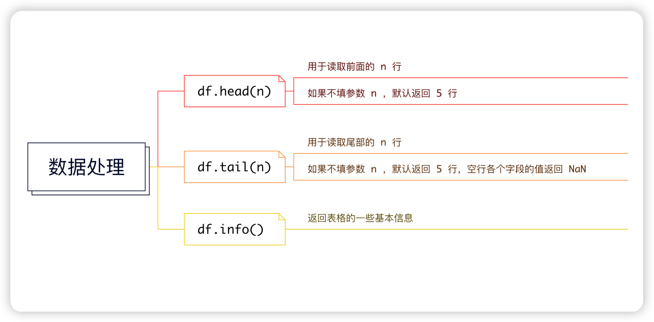
1:基本方法
1.1:Series的基本方法
| 方法 | 描述 |
|---|---|
axes |
返回行轴标签的列表 |
dtype |
返回对象的dtype。 |
empty |
如果Series为空,则返回True。 |
ndim |
根据定义返回基础数据的维数。 |
size |
返回基础数据中的元素数。 |
values |
将Series返回为ndarray。 |
head() |
返回前n行。 |
tail() |
返回最后n行。 |
python
import pandas as pd
import numpy as np

if __name__ == '__main__':
    ser = pd.Series(np.random.randn(4))
    print(ser)
    print(ser.axes)  # 返回轴标签的列表 [RangeIndex(start=0, stop=4, step=1)]
    print(ser.empty)  # 返回一个布尔值,判断该对象是否为空, 值为false
    print(ser.ndim)  # 返回维度,值为1
    print(ser.size)  # 返回元素个数,值为4
    print(ser.values) # 返回数组,值为[-0.37214805  0.35749305 -0.11696405  0.11696405]
    print(ser.head()) # 默认返回前5行数据,可以自定义数据
    print(ser.tail()) # 默认返回最后5行数据,可以自定义数据
1.2:DataFrame的基本方法
| 属性/方法 | 描述 |
|---|---|
T |
行和列互相转换 |
axes |
返回以行轴标签和列轴标签为唯一成员的列表。 |
dtypes |
返回此对象中的dtypes。 |
empty |
如果NDFrame完全为空没有项目,则为true;否则为false。如果任何轴的长度为0。 |
ndim |
轴数/数组尺寸。 |
shape |
返回表示DataFrame维度的元组。 |
size |
NDFrame中的元素数。 |
values |
NDFrame的数字表示。 |
head() |
返回前n行。 |
tail() |
返回最后n行。 |
python
import pandas as pd
import numpy as np

if __name__ == '__main__':
    d = {'Name': pd.Series(['A', 'B', 'C', 'D', 'E', 'F', 'G']),
         'Age': pd.Series([25, 26, 25, 23, 30, 29, 23]),
         'Rating': pd.Series([4.23, 3.24, 3.98, 2.56, 3.20, 4.6, 3.8])}
    # 创建一个 DataFrame
    df = pd.DataFrame(d)
    print(df)
    print("数据序列的转置是:")
    print(df.T)
    print("行轴标签和列轴标签是:")
    print(df.axes)
    print("每列的数据类型如下:")
    print(df.dtypes)
    print("Is the object empty?")
    print(df.empty)
    print("The dimension of the object is:")
    print(df.ndim)
    print("The shape of the object is:")
    print(df.shape)
    print("The total number of elements in our object is:")
    print(df.size)
    print("The actual data in our data frame is:")
    print(df.values)
    print("The first two rows of the data frame is:")
    print(df.head(2))
    print("The last two rows of the data frame is:")
print(df.tail(2)) Name Age Rating
0 A 25 4.23
1 B 26 3.24
2 C 25 3.98
3 D 23 2.56
4 E 30 3.20
5 F 29 4.60
6 G 23 3.80
数据序列的转置是:
0 1 2 3 4 5 6
Name A B C D E F G
Age 25 26 25 23 30 29 23
Rating 4.23 3.24 3.98 2.56 3.2 4.6 3.8
行轴标签和列轴标签是:
[RangeIndex(start=0, stop=7, step=1), Index(['Name', 'Age', 'Rating'], dtype='object')]
每列的数据类型如下:
Name object
Age int64
Rating float64
dtype: object
Is the object empty?
False
The dimension of the object is:
2
The shape of the object is:
(7, 3)
The total number of elements in our object is:
21
The actual data in our data frame is:
[['A' 25 4.23]
['B' 26 3.24]
['C' 25 3.98]
['D' 23 2.56]
['E' 30 3.2]
['F' 29 4.6]
['G' 23 3.8]]
The first two rows of the data frame is:
Name Age Rating
0 A 25 4.23
1 B 26 3.24
The last two rows of the data frame is:
Name Age Rating
5 F 29 4.6
6 G 23 3.82:描述性统计
DataFrame用在大量的计算描述性信息统计和其他相关操作。其中大多数是聚合,例如sum(),mean()
一般而言,这些方法采用轴参数,就像ndarray。{sum,std,...}一样,但是可以通过名称或整数指定轴
1.1:sum()
返回所请求轴的值之和。默认情况下,轴为索引(轴=0)
python
import pandas as pd
import numpy as np

d = {'Name':pd.Series(['A','B','C','D','E','F','G', 'H','I','J','K','L']),
    'Age':pd.Series([25,26,25,23,30,29,23,34,40,30,51,46]),
    'Rating':pd.Series([4.23,3.24,3.98,2.56,3.20,4.6,3.8,3.78,2.98,4.80,4.10,3.65])
 }

# 字典series -> dataframe
df = pd.DataFrame(d)

# 根据索引求和
print(df.sum())

print(df)/Users/cuihaida/project/python/first/venv/bin/python /Users/cuihaida/project/python/first/my-data-anaylze/my_pandas03.py
Name ABCDEFGHIJKL
Age 382
Rating 44.92
dtype: object
Name Age Rating
0 A 25 4.23
1 B 26 3.24
2 C 25 3.98
3 D 23 2.56
4 E 30 3.20
5 F 29 4.60
6 G 23 3.80
7 H 34 3.78
8 I 40 2.98
9 J 30 4.80
10 K 51 4.10
11 L 46 3.65
Process finished with exit code 01.2:mean()
返回平均值
python
import pandas as pd
import numpy as np

d = {'Name':pd.Series(['A','B','C','D','E','F','G', 'H','I','J','K','L']),
    'Age':pd.Series([25,26,25,23,30,29,23,34,40,30,51,46]),
    'Rating':pd.Series([4.23,3.24,3.98,2.56,3.20,4.6,3.8,3.78,2.98,4.80,4.10,3.65])
 }

# 字典series -> dataframe
df = pd.DataFrame(d)

# 根据索引求和
print(df.sum())
print("=" * 20)
print(df.sum(axis=1, numeric_only=True))  # age + rating
print("=" * 20)

# 返回平均值
print(df.mean(axis=0, skipna=True, numeric_only=True))
print("=" * 20)
print(df)/Users/cuihaida/project/python/first/venv/bin/python /Users/cuihaida/project/python/first/my-data-anaylze/my_pandas03.py
Name ABCDEFGHIJKL
Age 382
Rating 44.92
dtype: object
====================
0 29.23
1 29.24
2 28.98
3 25.56
4 33.20
5 33.60
6 26.80
7 37.78
8 42.98
9 34.80
10 55.10
11 49.65
dtype: float64
====================
Age 31.833333
Rating 3.743333
dtype: float64
====================
Name Age Rating
0 A 25 4.23
1 B 26 3.24
2 C 25 3.98
3 D 23 2.56
4 E 30 3.20
5 F 29 4.60
6 G 23 3.80
7 H 34 3.78
8 I 40 2.98
9 J 30 4.80
10 K 51 4.10
11 L 46 3.65
Process finished with exit code 01.3:其他统计性函数
| 编号 | 方法 | 描述 |
|---|---|---|
| 1 | count() |
非空数 |
| 2 | sum() |
总数 |
| 3 | mean() |
平均数 |
| 4 | median() |
中位数 |
| 5 | mode() |
模式 |
| 6 | std() |
标准差 |
| 7 | min() |
最低值 |
| 8 | max() |
最大值 |
| 9 | abs() |
绝对值 |
| 10 | prod() |
乘积 |
| 11 | cumsum() |
累加 |
| 12 | cumprod() |
累乘 |
由于DataFrame是异构数据结构。泛型运算并不适用于所有功能,注意下面两点:
- 诸如sum(),cumsum()之类的函数可用于数字和字符(或)字符串数据元素,而不会出现任何错误。虽然字符集合从不普遍使用,但不会抛出任何异常。
- 当DataFrame包含字符或字符串数据时,诸如abs(),cumprod()之类的函数将引发异常,因为此类操作无法执行。
1.4:汇总函数describe
此函数提供平均值,std和IQR值。并且,函数不包括字符列和有关数字列的给定摘要
同时这个函数还支持一个include参数,用于传递有关汇总时需要考虑哪些列的必要信息的参数。取值列表;默认情况下为"数字"。
- object − 汇总字符串列
- number − 汇总数字列
- all − 总结所有列在一起(不应该把它作为一个列表值)
python
import pandas as pd
import numpy as np

if __name__ == '__main__':
    d = {'Name': pd.Series(['A', 'B', 'C', 'D', 'E', 'F', 'G']),
         'Age': pd.Series([25, 26, 25, 23, 30, 29, 23]),
         'Rating': pd.Series([4.23, 3.24, 3.98, 2.56, 3.20, 4.6, 3.8])}
    df = pd.DataFrame(d)
    # 查看数据集的描述信息, include -> object,number,all
    # object -> object类型的数据, 就是字符串列
    # number -> 数值列, 默认
    # all -> 所有列
    print(df.describe(include=['number']))
3:函数的应用
要将您自己或其他库的函数应用于Pandas对象,您应该了解三个重要的方法:
- 表函数应用程序:pipe()
- 行或列函数应用程序:apply()
- 元素级函数应用程序:applymap()
要使用的适当方法取决于您的函数是希望对整个数据帧进行操作,还是行操作还是按列操作,还是按元素操作
3.1:表函数应用程序
可以通过传递函数和适当数量的参数作为管道参数来执行对DataFrame自定义操作,使用的方法是pipe()
python
import pandas as pd
import numpy as np

# 定义一个操作函数,到时候会让dataFrame应用这个函数
def adder(ele1, ele2):
    return ele1 + ele2

df = pd.DataFrame(np.random.randn(5,3),columns=['col1','col2','col3'])
print(df)
print("=" * 20)
ans = df.pipe(adder, 2) # 使用pipe()进行表函数应用, 对每一个元素 + 2
print(ans) col1 col2 col3
0 -1.743730 0.426996 -3.014761
1 0.209032 -0.407826 2.828854
2 -0.019639 0.879595 1.143649
3 0.155613 -0.562366 -3.301372
4 1.005468 -0.673557 -0.449234
====================
col1 col2 col3
0 0.256270 2.426996 -1.014761
1 2.209032 1.592174 4.828854
2 1.980361 2.879595 3.143649
3 2.155613 1.437634 -1.301372
4 3.005468 1.326443 1.5507663.2:行或列函数应用程序
可以使用apply()方法沿DataFrame或Panel的轴应用任意函数,该方法与描述性统计方法一样,采用可选的axis参数
默认情况下,该操作按列执行,将每一列视为类似数组的形式。
python
import pandas as pd
import numpy as np

# 定义一个操作函数,到时候会让dataFrame应用这个函数
def adder(ele1,ele2):
    return ele1+ele2

df = pd.DataFrame(np.random.randn(5,3),columns=['col1','col2','col3'])
print(df)
print(df.apply(np.mean)) # 列求平均
print(df.apply(np.mean,axis=1)) # 行求平均 col1 col2 col3
0 -0.123136 -0.512380 -0.258701
1 0.775471 -0.783096 -0.580526
2 -0.994060 -0.593498 -0.293823
3 -1.039347 0.523736 -0.062395
4 -0.378043 -0.651012 -0.509351
col1 -0.351823
col2 -0.403250
col3 -0.340959
dtype: float64
0 -0.298073
1 -0.196050
2 -0.627127
3 -0.192669
4 -0.512802
dtype: float643.3:元素级函数应用程序
并非所有函数都可以向量化(NumPy数组既不返回另一个数组,也不返回任何值)
DataFrame上的applymap() 方法和Series上的map() 类似地接受任何采用单个值并返回单个值的Python函数。
python
import pandas as pd
import numpy as np

df = pd.DataFrame(np.random.randn(5, 3), columns=['col1', 'col2', 'col3'])
# 自定义函数
print(df)
print("=" * 20)
print(df['col1'].map(lambda x: x + 100)) # 对col1列的每一个数进行加1操作,不会影响原数组 col1 col2 col3
0 0.720981 -1.848660 -1.021995
1 -0.263746 0.328287 -1.218116
2 -0.041258 0.364516 -0.553747
3 -0.772308 0.542454 -0.385765
4 -1.347373 -0.311151 0.608969
====================
0 100.720981
1 99.736254
2 99.958742
3 99.227692
4 98.652627
Name: col1, dtype: float644:重建索引
4.1:reindex()
重建索引 会更改DataFrame的行标签和列标签。重新索引是指使数据与特定轴上的一组给定标签匹配。
通过索引可以完成多个操作,例如:
-
重新排序现有数据以匹配一组新标签。
-
在标签数据不存在的标签位置中插入缺失值(NA)标记。
python
import pandas as pd
import numpy as np
N=20
df = pd.DataFrame({
    'A': pd.date_range(start='2016-01-01',periods=N,freq='D'),
    'x': np.linspace(0,stop=N-1,num=N),
    'y': np.random.rand(N),
    'C': np.random.choice(['Low','Medium','High'],N).tolist(),
    'D': np.random.normal(100, 10, size=(N)).tolist()
})

# DataFrame重建索引
# 找出df中的A, C, B列作为新的索引和列, 对于在df中不存在的列,默认填充NaN
df_reindexed = df.reindex(index=[0,2,5], columns=['A', 'C', 'B'])
print(df_reindexed) A C B
0 2016-01-01 Medium NaN
2 2016-01-03 Low NaN
5 2016-01-06 Low NaN4.2:reindex_like()
可以使用reindex_like()重新索引以与其他对象对齐
python
import pandas as pd
import numpy as np

def test2():
    df1 = pd.DataFrame(np.random.randn(10, 3), columns=['col1', 'col2', 'col3'])
    df2 = pd.DataFrame(np.random.randn(7, 3), columns=['col1', 'col2', 'col3'])
    df1 = df1.reindex_like(df2) # df1变成df2的索引和列的结构,也是7行3列,如果多出来就切断,如果少,就填充NaN
    print(df1)

if __name__ == '__main__':
test2() col1 col2 col3
0 -0.224233 1.808778 0.105156
1 -0.729603 0.874080 0.470185
2 -1.795519 0.289359 -1.302235
3 -1.007448 -0.064831 -0.150167
4 0.694548 0.283895 0.574875
5 0.410779 -1.394223 0.376044
6 -0.447436 1.297874 0.764893🎉 当然可以不填充NaN, 可以通过给reindex() & reindex_like()赋值method属性,决定填充信息
pad/ffill− 向前填充值bfill/backfill− 向后填充值nearest− 从最接近的索引值填充
🎉 在指定填充信息之后,还可以使用limit属性决定最多填充几行
python
import pandas as pd
import numpy as np

def test3():
    df1 = pd.DataFrame(np.random.randn(6, 3), columns=['col1', 'col2', 'col3'])
    df2 = pd.DataFrame(np.random.randn(2, 3), columns=['col1', 'col2', 'col3'])
    # 填充 NAN
    print(df2.reindex_like(df1))
    # 现在用前面的值填充NAN
    print("带前向填充的数据帧:")
    print(df2.reindex_like(df1, method='ffill'), limit=2) # 向前填充,最多填充2行

if __name__ == '__main__':
test3() col1 col2 col3
0 0.342667 0.725107 -0.40085
1 -0.346052 0.070069 -0.03319
2 NaN NaN NaN
3 NaN NaN NaN
4 NaN NaN NaN
5 NaN NaN NaN
带前向填充的数据帧:
col1 col2 col3
0 0.342667 0.725107 -0.40085
1 -0.346052 0.070069 -0.03319
2 -0.346052 0.070069 -0.03319
3 -0.346052 0.070069 -0.03319
4 NaN NaN NaN
5 NaN NaN NaN4.3:重命名
通过rename()方法,您可以基于某些映射(字典或系列)或任意函数来重新标记轴
python
import pandas as pd
import numpy as np

def test4():
    df1 = pd.DataFrame(np.random.randn(6, 3), columns=['col1', 'col2', 'col3'])
    print(df1)
    print("重命名行和列之后:")
    new = df1.rename(columns={'col1': 'c1', 'col2': 'c2'}, index={0: 'foo', 1: 'bar'})
    print(new)

if __name__ == '__main__':
test4() col1 col2 col3
0 1.985762 1.067307 -0.681527
1 0.240389 0.700743 0.051090
2 -1.677559 0.175037 0.242483
3 0.623115 -0.200200 0.216992
4 2.097055 -1.563505 -0.156450
5 0.672499 0.088381 -0.601609
重命名行和列之后:
c1 c2 col3
foo 1.985762 1.067307 -0.681527
bar 0.240389 0.700743 0.051090
2 -1.677559 0.175037 0.242483
3 0.623115 -0.200200 0.216992
4 2.097055 -1.563505 -0.156450
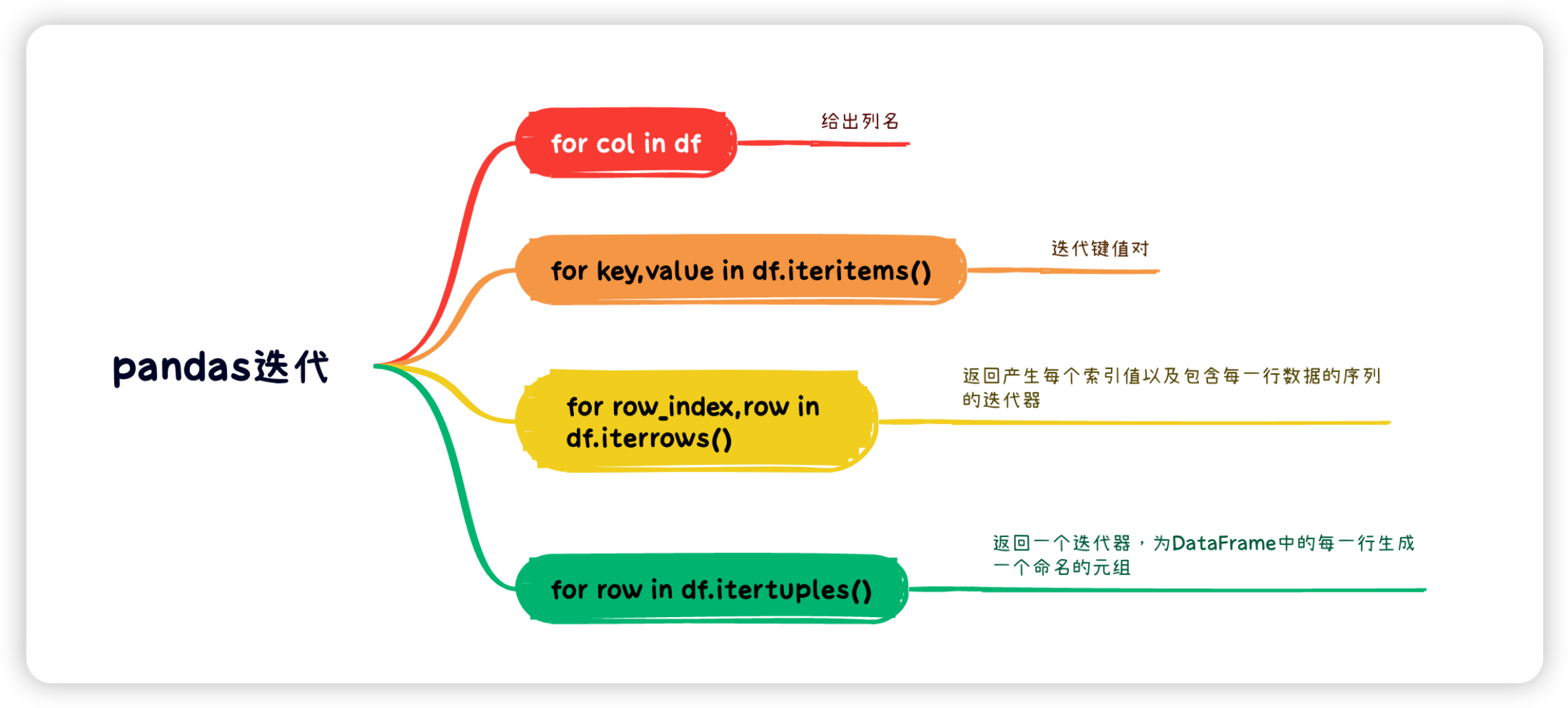
5 0.672499 0.088381 -0.6016095:迭代和排序
5.1:迭代
5.2:排序
核心就是sort_index()和sort_values()
python
import numpy as np
import pandas as pd

def test1():
    # 定义一个10行两列的dataframe, index表示每一行的索引,columns表示每一列的key
    unsorted_df = pd.DataFrame(np.random.randn(10, 2), index=[1, 4, 6, 2, 3, 5, 9, 8, 0, 7], columns = ['col2', 'col1'])
    print(unsorted_df)
    print("默认排序")
    print(unsorted_df.sort_index()) # 排序, 默认根据index的升序排序(index从0 -> 9)
    print("可以使用ascending参数控制倒排")
    print(unsorted_df.sort_index(ascending=False))  # 倒排, index从9 -> 0
    print("也可以对列进行排序, 可以通过指定axis = 1")
    print(unsorted_df.sort_index(axis=1))
    print("可以使用 sort_values() 对值进行排序, by属性是通过那个key, 可以指定多个,列表形式")
    print(unsorted_df.sort_values(by='col1'))
    print("sort_values() 提供了从mergesort归并排序,heapsort堆排序和quicksort快排中选择算法的指定")
    print("mergesort是唯一稳定的排序")
    print(unsorted_df.sort_values(by='col1', kind='mergesort'))


if __name__ == '__main__':
test1()/Users/cuihaida/project/python/first/venv/bin/python /Users/cuihaida/project/python/first/my-data-anaylze/my_pandas04.py
col2 col1
1 0.071396 -1.011856
4 -0.218280 0.530760
6 -0.206268 0.562001
2 -0.385724 2.792641
3 -0.294598 -0.322529
5 -0.212050 0.278547
9 0.375532 -0.281603
8 0.690356 1.799434
0 -0.974060 -1.411210
7 0.502817 0.433678
默认排序
col2 col1
0 -0.974060 -1.411210
1 0.071396 -1.011856
2 -0.385724 2.792641
3 -0.294598 -0.322529
4 -0.218280 0.530760
5 -0.212050 0.278547
6 -0.206268 0.562001
7 0.502817 0.433678
8 0.690356 1.799434
9 0.375532 -0.281603
可以使用ascending参数控制倒排
col2 col1
9 0.375532 -0.281603
8 0.690356 1.799434
7 0.502817 0.433678
6 -0.206268 0.562001
5 -0.212050 0.278547
4 -0.218280 0.530760
3 -0.294598 -0.322529
2 -0.385724 2.792641
1 0.071396 -1.011856
0 -0.974060 -1.411210
也可以对列进行排序, 可以通过指定axis = 1
col1 col2
1 -1.011856 0.071396
4 0.530760 -0.218280
6 0.562001 -0.206268
2 2.792641 -0.385724
3 -0.322529 -0.294598
5 0.278547 -0.212050
9 -0.281603 0.375532
8 1.799434 0.690356
0 -1.411210 -0.974060
7 0.433678 0.502817
可以使用 sort_values() 对值进行排序, by属性是通过那个key, 可以指定多个,列表形式
col2 col1
0 -0.974060 -1.411210
1 0.071396 -1.011856
3 -0.294598 -0.322529
9 0.375532 -0.281603
5 -0.212050 0.278547
7 0.502817 0.433678
4 -0.218280 0.530760
6 -0.206268 0.562001
8 0.690356 1.799434
2 -0.385724 2.792641
sort_values() 提供了从mergesort归并排序,heapsort堆排序和quicksort快排中选择算法的指定
mergesort是唯一稳定的排序
col2 col1
0 -0.974060 -1.411210
1 0.071396 -1.011856
3 -0.294598 -0.322529
9 0.375532 -0.281603
5 -0.212050 0.278547
7 0.502817 0.433678
4 -0.218280 0.530760
6 -0.206268 0.562001
8 0.690356 1.799434
2 -0.385724 2.792641
Process finished with exit code 06:series的文本处理
几乎所有这些方法都可用于Python字符串函数
因此,将Series对象转换为String对象,然后执行该操作。
| 方法 | 说明 |
|---|---|
lower() |
将系列/索引中的字符串转换为小写。 |
upper() |
将系列/索引中的字符串转换为大写。 |
len() |
计算字符串length()。 |
strip() |
帮助从两侧从系列/索引中的每个字符串中去除空格(包括换行符)。 |
split(' ') |
用给定的模式分割每个字符串。 |
cat(sep=' ') |
用给定的分隔符连接系列/索引元素。 |
get_dummies() |
返回具有一键编码值的DataFrame。 |
contains(pattern) |
如果子字符串包含在元素中,则为每个元素返回一个布尔值True,否则返回False。 |
replace(a,b) |
a值替换成b。 |
repeat(value) |
以指定的次数重复每个元素。 |
count(pattern) |
返回每个元素中模式出现的次数。 |
startswith(pattern) |
如果系列/索引中的元素以模式开头,则返回true。 |
endswith(pattern) |
如果系列/索引中的元素以模式结尾,则返回true。 |
find(pattern) |
返回模式首次出现的第一个位置。 |
findall(pattern) |
返回所有出现的模式的列表。 |
swapcase |
大小写互换 |
islower() |
检查"系列/索引"中每个字符串中的所有字符是否都小写。返回布尔值 |
isupper() |
检查"系列/索引"中每个字符串中的所有字符是否都大写。返回布尔值。 |
isnumeric() |
检查"系列/索引"中每个字符串中的所有字符是否都是数字。返回布尔值。 |
python
import numpy as np
import pandas as pd
def test2():
s = pd.Series(['Tom', 'William Rick', 'John', 'Alber@t', np.nan, '1234', 'SteveSmith'])
print(s.str.len())
print(s.str.lower())
print(s.str.upper())
if __name__ == '__main__':
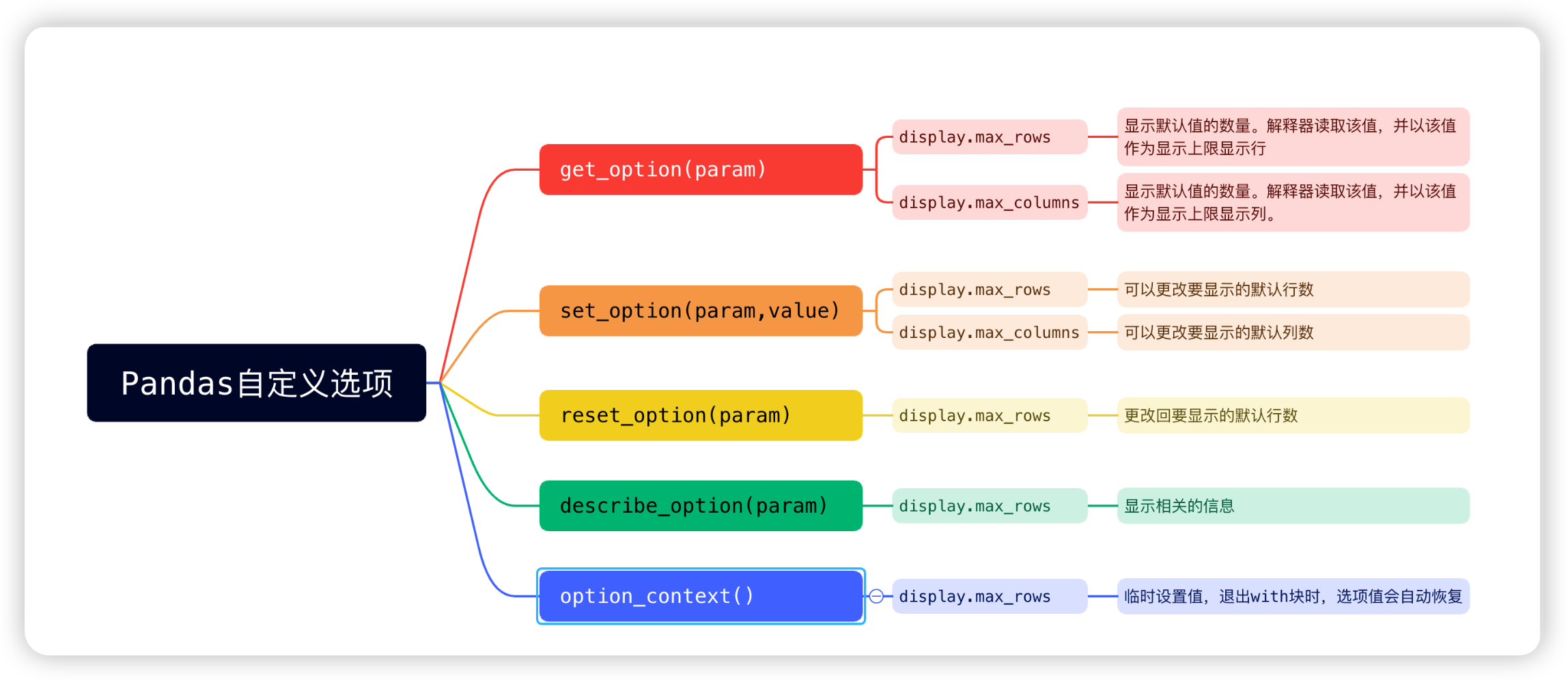
test2()7:自定义选项的设置
python
import numpy as np
import pandas as pd

def test3():
    # 查看可以展示的最大行数和列数
    print(pd.get_option("display.max_rows"))
    print(pd.get_option("display.max_columns"))  # 默认显示的列数是0, 表示显示所有列
    print("=" * 40)
    # 设置最大行数和列数
    pd.set_option("display.max_rows", 10)
    pd.set_option("display.max_columns", 10)  # 调整成为最多显示10列
    print(pd.get_option("display.max_rows"))
    print(pd.get_option("display.max_columns"))
    print("=" * 40)
    # 恢复默认
    pd.reset_option("display.max_rows")
    pd.reset_option("display.max_columns")
    print(pd.get_option("display.max_rows"))
    print(pd.get_option("display.max_columns"))
    print("=" * 40)
    # 查看描述
    print(pd.describe_option("display.max_rows"))
    print(pd.describe_option("display.max_columns"))
    print("=" * 40)
    # 临时设置,只在with块中生效
    with pd.option_context("display.max_rows", 10, "display.max_columns", 10):
        print(pd.get_option("display.max_rows"))  # 10
        print(pd.get_option("display.max_columns"))  # 10
        print("=" * 40)
    print(pd.get_option("display.max_rows")) # 60, 不受到option_context的设置的影响
    print(pd.get_option("display.max_columns")) # 10
    print("=" * 40)

if __name__ == '__main__':
test3()60
0
========================================
10
10
========================================
60
0
========================================
display.max_rows : int
If max_rows is exceeded, switch to truncate view. Depending on
`large_repr`, objects are either centrally truncated or printed as
a summary view. 'None' value means unlimited.
In case python/IPython is running in a terminal and `large_repr`
equals 'truncate' this can be set to 0 and pandas will auto-detect
the height of the terminal and print a truncated object which fits
the screen height. The IPython notebook, IPython qtconsole, or
IDLE do not run in a terminal and hence it is not possible to do
correct auto-detection.
[default: 60] [currently: 60]
None
display.max_columns : int
If max_cols is exceeded, switch to truncate view. Depending on
`large_repr`, objects are either centrally truncated or printed as
a summary view. 'None' value means unlimited.
In case python/IPython is running in a terminal and `large_repr`
equals 'truncate' this can be set to 0 or None and pandas will auto-detect
the width of the terminal and print a truncated object which fits
the screen width. The IPython notebook, IPython qtconsole, or IDLE
do not run in a terminal and hence it is not possible to do
correct auto-detection and defaults to 20.
[default: 0] [currently: 0]
None
========================================
10
10
========================================
60
0
========================================8:索引和数据查询
Python和NumPy索引运算符"\[\]"和属性运算符"."。可以在各种用例中快速轻松地访问Pandas数据结构
Pandas现在支持两种类型的多轴索引:下表中提到了三种类型:
| 索引 | 说明 |
|---|---|
.loc() |
基于标签 |
.iloc() |
基于整数 |
8.1:loc
.loc() 具有多种访问方法,例如:
- 一个标量标签
- 标签列表
- 切片对象
- 布尔数组
loc 需要两个单/列表/范围运算符,以","分隔。第一个指示行,第二个指示列。
python
import pandas as pd
import numpy as np

def test1():
    df = pd.DataFrame(np.random.randn(8, 4),
                      index=['a', 'b', 'c', 'd', 'e', 'f', 'g', 'h'],
                      columns=['A', 'B', 'C', 'D'])  # 定义一个8行4列的DataFrame, 索引为a-h, 列名为A-D
    print(df)
    print("筛选出每一行的A列")
    print(df['A'])
    print("=" * 30)
    print(df.loc[:, 'A'])
    print("=" * 30)
    print("筛选出所有的AC列")
    print(df.loc[:, ['A', 'C']])
    print("=" * 30)
    print("同时可以指定行和列, 例如输出a, c, f行的A, C列")
    print(df.loc[['a', 'c', 'f'], ['A', 'C']])
    print("=" * 30)
    print("可以为所有的列指定行的范围,使用:")
    print(df.loc['a':'c', ['A', 'C']])
    print("=" * 30)

if __name__ == '__main__':
test1() A B C D
a 1.382366 -1.163601 0.176177 0.672256
b -0.282480 -0.967808 0.930259 0.316234
c -0.043770 1.639644 -0.505511 1.421071
d 0.660928 0.612623 0.292144 1.240187
e 1.449997 -0.061115 0.104454 0.194620
f -1.048595 -0.017617 0.250532 -1.888130
g 0.856651 0.994930 -0.220943 1.727685
h -0.482508 -0.440425 -0.317698 -0.555271
筛选出每一行的A列
a 1.382366
b -0.282480
c -0.043770
d 0.660928
e 1.449997
f -1.048595
g 0.856651
h -0.482508
Name: A, dtype: float64
==============================
a 1.382366
b -0.282480
c -0.043770
d 0.660928
e 1.449997
f -1.048595
g 0.856651
h -0.482508
Name: A, dtype: float64
==============================
筛选出所有的AC列
A C
a 1.382366 0.176177
b -0.282480 0.930259
c -0.043770 -0.505511
d 0.660928 0.292144
e 1.449997 0.104454
f -1.048595 0.250532
g 0.856651 -0.220943
h -0.482508 -0.317698
==============================
同时可以指定行和列, 例如输出a, c, f行的A, C列
A C
a 1.382366 0.176177
c -0.043770 -0.505511
f -1.048595 0.250532
==============================
可以为所有的列指定行的范围,使用:
A C
a 1.382366 0.176177
b -0.282480 0.930259
c -0.043770 -0.505511
==============================8.2:iloc
同理,只不过这个索引切片变成了整数
python
import pandas as pd
import numpy as np

def test2():
    df = pd.DataFrame(np.random.randn(8, 4),
                      index=['a', 'b', 'c', 'd', 'e', 'f', 'g', 'h'],
                      columns=['A', 'B', 'C', 'D'])
    print(df)
    print("=" * 30)
    print("df中的前4行是:")
    print(df.iloc[:4])
    print("=" * 30)
    print("df中的后4行是:")
    print(df.iloc[4:])
    print("=" * 30)
    print("df中的第2行和第4行是:")
    print(df.iloc[[1, 3]])
    print("=" * 30)
    print("df中的前4行的后两列是:")
    print(df.iloc[:4, 2:])
    print("=" * 30)
    print("df中的第2行和第4行,第2列和第4列是:")
    print(df.iloc[[1, 3], [1, 3]])
    print("=" * 30)

if __name__ == '__main__':
test2() A B C D
a -0.343237 -0.155287 -0.713359 0.071921
b -0.165145 0.491577 -0.107699 1.016831
c -0.527483 -0.391398 0.700065 0.054806
d -2.306590 0.223241 -0.097838 -0.431856
e -1.398431 -0.267630 0.366289 -0.373675
f -0.446961 -1.622479 -0.319882 -0.999932
g 0.645857 -1.249595 0.513613 -0.140469
h 0.227319 0.543510 1.938501 1.312588
==============================
df中的前4行是:
A B C D
a -0.343237 -0.155287 -0.713359 0.071921
b -0.165145 0.491577 -0.107699 1.016831
c -0.527483 -0.391398 0.700065 0.054806
d -2.306590 0.223241 -0.097838 -0.431856
==============================
df中的后4行是:
A B C D
e -1.398431 -0.267630 0.366289 -0.373675
f -0.446961 -1.622479 -0.319882 -0.999932
g 0.645857 -1.249595 0.513613 -0.140469
h 0.227319 0.543510 1.938501 1.312588
==============================
df中的第2行和第4行是:
A B C D
b -0.165145 0.491577 -0.107699 1.016831
d -2.306590 0.223241 -0.097838 -0.431856
==============================
df中的前4行的后两列是:
C D
a -0.713359 0.071921
b -0.107699 1.016831
c 0.700065 0.054806
d -0.097838 -0.431856
==============================
df中的第2行和第4行,第2列和第4列是:
B D
b 0.491577 1.016831
d 0.223241 -0.431856
==============================四:高级操作
1:缺失值处理
1.1:对于缺失值的表示
- NaN :
float类型的默认缺失标记(来自 NumPy) - None :
object类型的缺失标记(Python 内置) - NaT :时间类型(
datetime64)的缺失值
1.2:对于缺失值的检测
python
df.isna()       # 返回布尔矩阵(True=缺失)
df.notna()      # 返回布尔矩阵(False=缺失)
df.isnull()     # isna() 的别名(功能相同)

df.isna().sum()             # 每列缺失值数量
df.isna().sum().sum()       # 整个DataFrame缺失值总数
df.isna().mean() * 100      # 每列缺失值百分比
python
import numpy as np
import pandas as pd

dict = {
    'name': ['Tom', 'Nick', 'John'],
    'age': [20, 21, 19],
    'city': ['New York', 'Paris', None]
}

df = pd.DataFrame(dict)

print(df)
print("=" * 50)
print("布尔矩阵,如果是缺失值,将返回True, 否则是False")
print(df.isna())
print("=" * 50)
print("每列缺失值百分比")
print(df.isna().mean() * 100)
1.3:对于缺失值的删除
python
# 删除包含缺失值的行(默认)
df.dropna(axis=0)

# 删除包含缺失值的列
df.dropna(axis=1)

# 删除全为缺失值的行
df.dropna(how='all')

# 删除在特定列有缺失的行
df.dropna(subset=['col1', 'col2'])

# 保留至少有 n 个非缺失值的行
df.dropna(thresh=5)
1.4:对于缺失值的填充
python
# 可以固定值填充
df.fillna(0)  # 所有缺失值填充为0
df.fillna({'col1': 0, 'col2': 'unknown'})  # 按列指定填充值

# 统计值填充
df.fillna(df.mean()) # 用各列均值填充
df['col1'].fillna(df['col1'].median(), inplace=True)  # 中位数填充(原地修改)

# 前后填充
df.fillna(method='ffill')      # 用前一个有效值填充(向前填充)
df.fillna(method='bfill')      # 用后一个有效值填充(向后填充)
df.fillna(method='ffill', limit=2)  # 最多向前填充2个

# 插值法填充
df.interpolate()               # 线性插值(默认)
df.interpolate(method='time')  # 时间索引插值
df.interpolate(method='polynomial', order=2)  # 二阶多项式插值
1.5:其他常用操作
python
# 将数值列的NaN替换为None(转换类型)
df['col'] = df['col'].where(pd.notnull(df['col']), None)

# 按分组用组内均值填充
df.groupby('group_col').transform(lambda x: x.fillna(x.mean()))

# 将占位符(如 -999)识别为缺失值
df.replace(-999, np.nan, inplace=True)
2:统计、分组和连接
Pandas核心操作 统计计算 分组操作 数据连接 描述性统计 相关性分析 分布分析 累积计算 分组聚合 分组转换 分组过滤 分组迭代 Merge合并 Join连接 Concatenate拼接 数据比较 高级技巧 透视表 交叉表 时间重采样 性能优化
2.1:统计计算
基础统计函数
python
import pandas as pd
import numpy as np

# 创建示例数据
data = {
    'Product': ['A', 'B', 'C', 'D', 'E'],
    'Sales': [250, 300, 180, 400, np.nan],
    'Cost': [120, 150, 100, 220, 180],
    'Category': ['Electronics', 'Furniture', 'Electronics', 'Furniture', 'Office']
}
df = pd.DataFrame(data)

# 基本统计信息
print("描述性统计:")
print(df.describe())

# 特定统计计算
print("\n销售总额:", df['Sales'].sum())
print("平均成本:", df['Cost'].mean())
print("最大销售额:", df['Sales'].max())
print("销售额标准差:", df['Sales'].std())
print("非空值数量:", df['Sales'].count())
相关性的分析
python
import pandas as pd
import numpy as np

# 创建示例数据
data = {
    'Product': ['A', 'B', 'C', 'D', 'E'],
    'Sales': [250, 300, 180, 400, np.nan],
    'Cost': [120, 150, 100, 220, 180],
    'Category': ['Electronics', 'Furniture', 'Electronics', 'Furniture', 'Office']
}
df = pd.DataFrame(data)

# 添加利润列
df['Profit'] = df['Sales'] - df['Cost']

# 计算相关性矩阵
correlation = df[['Sales', 'Cost', 'Profit']].corr()
print("\n相关性矩阵:")
print(correlation)

# 单个相关性
print("\n销售与利润的相关性:", df['Sales'].corr(df['Profit']))
累积计算
python
import pandas as pd
import numpy as np

# 创建示例数据
data = {
    'Product': ['A', 'B', 'C', 'D', 'E'],
    'Sales': [250, 300, 180, 400, np.nan],
    'Cost': [120, 150, 100, 220, 180],
    'Category': ['Electronics', 'Furniture', 'Electronics', 'Furniture', 'Office']
}
df = pd.DataFrame(data)

# 累积计算
df['Cumulative_Sales'] = df['Sales'].cumsum()  # 累积求和, [250, 550, 730, 1130]
df['Running_Max'] = df['Sales'].cummax()  # 累积最大值, [250, 300, 300, 400]

print("\n累积统计:")
print(df[['Product', 'Sales', 'Cumulative_Sales', 'Running_Max']])()

print("\n累积统计:")
print(df[['Product', 'Sales', 'Cumulative_Sales', 'Running_Max']])
分布分析
python
import pandas as pd
import numpy as np

# 创建示例数据
data = {
    'Product': ['A', 'B', 'C', 'D', 'E'],
    'Sales': [250, 300, 180, 400, np.nan],
    'Cost': [120, 150, 100, 220, 180],
    'Category': ['Electronics', 'Furniture', 'Electronics', 'Furniture', 'Office']
}
df = pd.DataFrame(data)

# 值计数
print("\n类别分布:")
print(df['Category'].value_counts())

# 分位数
print("\n销售额的25%分位数:", df['Sales'].quantile(0.25))
print("销售额的50%分位数:", df['Sales'].quantile(0.5))

# 直方图分箱
print("\n销售额分布:")
print(pd.cut(df['Sales'], bins=3).value_counts())
2.2:分组操作
基础分组统计
python
import pandas as pd
import numpy as np

# 创建示例数据
data = {
    'Product': ['A', 'B', 'C', 'D', 'E'],
    'Sales': [250, 300, 180, 400, np.nan],
    'Cost': [120, 150, 100, 220, 180],
    'Category': ['Electronics', 'Furniture', 'Electronics', 'Furniture', 'Office']
}
df = pd.DataFrame(data)
# 按类别分组并计算平均值
category_group = df.groupby('Category')
print("\n按类别分组平均值:")
print(category_group.mean(numeric_only=True))

# 多列分组
multi_group = df.groupby(['Category', 'Product'])
print("\n多级分组总和:")
print(multi_group.sum(numeric_only=True))
聚合函数
python
import pandas as pd
import numpy as np

# 创建示例数据
data = {
    'Product': ['A', 'B', 'C', 'D', 'E'],
    'Sales': [250, 300, 180, 400, np.nan],
    'Cost': [120, 150, 100, 220, 180],
    'Category': ['Electronics', 'Furniture', 'Electronics', 'Furniture', 'Office']
}
df = pd.DataFrame(data)
# 应用多个聚合函数
agg_results = category_group.agg({
    'Sales': ['sum', 'mean', 'max'],
    'Cost': ['min', 'median']
})
print("\n多聚合函数结果:")
print(agg_results)
分组转换
python
import pandas as pd
import numpy as np

# 创建示例数据
data = {
    'Product': ['A', 'B', 'C', 'D', 'E'],
    'Sales': [250, 300, 180, 400, np.nan],
    'Cost': [120, 150, 100, 220, 180],
    'Category': ['Electronics', 'Furniture', 'Electronics', 'Furniture', 'Office']
}
df = pd.DataFrame(data)
# 计算组内标准化值
df['Z-Score'] = category_group['Sales'].transform(
    lambda x: (x - x.mean()) / x.std()
)

# 填充组内平均值
df['Sales_Filled'] = category_group['Sales'].transform(
    lambda x: x.fillna(x.mean())
)

print("\n分组转换结果:")
print(df[['Product', 'Category', 'Sales', 'Z-Score', 'Sales_Filled']])
分组过滤
python
import pandas as pd
import numpy as np

# 创建示例数据
data = {
    'Product': ['A', 'B', 'C', 'D', 'E'],
    'Sales': [250, 300, 180, 400, np.nan],
    'Cost': [120, 150, 100, 220, 180],
    'Category': ['Electronics', 'Furniture', 'Electronics', 'Furniture', 'Office']
}
df = pd.DataFrame(data)

# 过滤销售总额超过400的组
filtered_groups = category_group.filter(lambda x: x['Sales'].sum() > 400)
print("\n销售总额超过400的类别:")
print(filtered_groups)
分组迭代
python
import pandas as pd
import numpy as np

# 创建示例数据
data = {
    'Product': ['A', 'B', 'C', 'D', 'E'],
    'Sales': [250, 300, 180, 400, np.nan],
    'Cost': [120, 150, 100, 220, 180],
    'Category': ['Electronics', 'Furniture', 'Electronics', 'Furniture', 'Office']
}
df = pd.DataFrame(data)

category_group = df.groupby('Category')

print("\n分组迭代:")
for name, group in category_group:
    print(f"\n类别: {name}")
    print(group[['Product', 'Sales']])
2.3:数据连接
合并 (Merge)
python
# 创建第二个DataFrame
inventory = pd.DataFrame({
    'Product': ['A', 'B', 'C', 'F'],
    'Stock': [15, 8, 20, 12],
    'Warehouse': ['NY', 'CA', 'TX', 'FL']
})

# 内连接
inner_merge = pd.merge(df, inventory, on='Product', how='inner')
print("\n内连接结果:")
print(inner_merge)

# 左连接
left_merge = pd.merge(df, inventory, on='Product', how='left')
print("\n左连接结果:")
print(left_merge)

# 指定不同列名
prices = pd.DataFrame({
    'Item': ['A', 'B', 'C', 'D', 'E'],
    'Price': [99, 149, 79, 199, 129]
})
different_cols = pd.merge(df, prices, left_on='Product', right_on='Item')
print("\n不同列名连接:")
print(different_cols[['Product', 'Sales', 'Price']])
连接 (Join)
python
# 设置索引
df_indexed = df.set_index('Product')
inventory_indexed = inventory.set_index('Product')

# 索引连接
joined = df_indexed.join(inventory_indexed, how='left')
print("\n索引连接结果:")
print(joined)
拼接 (Concatenate)
python
# 创建新数据
new_products = pd.DataFrame({
    'Product': ['F', 'G'],
    'Sales': [320, 280],
    'Cost': [150, 130],
    'Category': ['Electronics', 'Office']
})

# 垂直拼接
vertical_concat = pd.concat([df, new_products], ignore_index=True)
print("\n垂直拼接结果:")
print(vertical_concat)

# 水平拼接
additional_info = pd.DataFrame({
    'Product': ['A', 'B', 'C', 'D', 'E'],
    'Rating': [4.5, 4.2, 4.8, 4.0, 4.6]
})
horizontal_concat = pd.concat([df, additional_info.set_index('Product')], axis=1)
print("\n水平拼接结果:")
print(horizontal_concat)
比较与组合
python
# 比较数据集
comparison = df.compare(new_products)
print("\n数据集比较:")
print(comparison)

# 组合数据
combine_first = df.set_index('Product').combine_first(
    new_products.set_index('Product')
)
print("\n组合数据结果:")
print(combine_first)
2.4:高级技巧
数据透视表
python
# 创建透视表
pivot_table = pd.pivot_table(
    df,
    values='Sales',
    index='Category',
    columns=pd.cut(df['Cost'], bins=[0, 150, 250]),
    aggfunc=['sum', 'mean'],
    fill_value=0
)
print("\n数据透视表:")
print(pivot_table)
交叉表
python
# 创建交叉表
cross_tab = pd.crosstab(
    df['Category'],
    pd.cut(df['Cost'], bins=[0, 150, 250]),
    values=df['Sales'],
    aggfunc='mean'
)
print("\n交叉表:")
print(cross_tab)
分组时间序列重采样
python
# 创建时间序列数据
date_rng = pd.date_range(start='2023-01-01', end='2023-01-10', freq='D')
time_series = pd.DataFrame({
    'Date': date_rng,
    'Sales': np.random.randint(100, 500, size=(len(date_rng))),
    'Category': np.random.choice(['Electronics', 'Furniture', 'Office'], size=len(date_rng))
})

# 按类别分组并重采样
time_series.set_index('Date', inplace=True)
resampled = time_series.groupby('Category').resample('3D').sum()
print("\n时间序列重采样:")
print(resampled)
3:日期相关操作
3.1:日期的创建和转换
创建时间戳
python
ts = pd.Timestamp("2023-08-15 14:30:00")
print("单个时间戳", ts)

# 时间范围, periods -> 个数, freq -> 时间间隔,D-天,H-小时,M-分钟,S-秒
date_range = pd.date_range('2023-01-01', periods=5, freq='D')
print("\n日期范围:", date_range)

# 工作日范围(bdate)
bdate_range = pd.bdate_range('2023-08-01', periods=5)
print("\n工作日范围:", bdate_range)
转换数据类型
python
# 从字符串转换
dates = ['2023-01-01', '2023-02-15', '2023-03-22']
df = pd.DataFrame({'date_str': dates})
df['date_dt'] = pd.to_datetime(df['date_str'])
print("\n字符串转日期:\n", df)

# 从不同格式转换
euro_dates = ['15/08/2023', '20/09/2023', '05/11/2023']
df['euro_date'] = pd.to_datetime(euro_dates, format='%d/%m/%Y')
print("\n欧洲格式日期:\n", df)

# 处理错误日期
mixed_dates = ['2023-01-01', 'invalid', '2023-03-22', '2023-02-30']
df = pd.DataFrame({'date': mixed_dates})
df['converted'] = pd.to_datetime(df['date'], errors='coerce')
print("\n错误处理转换:\n", df)
3.2:日期时间属性提取
dt.year/month/day/...
基本属性的提取
python
# 创建时间序列数据
dates = pd.date_range('2023-01-01', periods=10, freq='D')
df = pd.DataFrame({'date': dates})

# 提取日期组件
df['year'] = df['date'].dt.year
df['month'] = df['date'].dt.month
df['day'] = df['date'].dt.day
df['dayofweek'] = df['date'].dt.dayofweek  # 周一=0, 周日=6
df['day_name'] = df['date'].dt.day_name()
df['is_weekend'] = df['date'].dt.dayofweek >= 5

print("\n日期属性提取:\n", df.head())
时间属性的提取
python
# 创建带时间的数据
times = pd.date_range('2023-01-01 08:00', periods=5, freq='4H')
df = pd.DataFrame({'datetime': times})

# 提取时间组件
df['hour'] = df['datetime'].dt.hour
df['minute'] = df['datetime'].dt.minute
df['second'] = df['datetime'].dt.second
df['time'] = df['datetime'].dt.time
df['period'] = pd.cut(df['hour'],
                     bins=[0, 6, 12, 18, 24],
                     labels=['Night', 'Morning', 'Afternoon', 'Evening'])

print("\n时间属性提取:\n", df)
3.3:日期时间运算
时间差的计算
python
# 创建时间差
td1 = pd.Timedelta(days=5, hours=3)
print("\n时间差:", td1)

# 时间运算
start = pd.Timestamp('2023-01-01')
end = start + pd.Timedelta(weeks=2)
print("开始日期:", start)
print("结束日期:", end)
print("时间差:", end - start)

# 序列运算
dates = pd.date_range('2023-01-01', periods=5, freq='2D')
df = pd.DataFrame({'date': dates})
df['next_date'] = df['date'] + pd.Timedelta(days=1)
df['days_diff'] = (df['next_date'] - df['date']).dt.days

print("\n时间差计算:\n", df)
日期的偏移
python
from pandas.tseries.offsets import *

# 基本偏移
date = pd.Timestamp('2023-08-15')
print("\n原始日期:", date)
print("加3天:", date + DateOffset(days=3))
print("加2个月:", date + DateOffset(months=2))

# 工作日偏移
print("下个工作日:", date + BDay())
print("下个月第一个工作日:", date + BMonthBegin())

# 特殊偏移
print("季度末:", date + BQuarterEnd())
print("财年末(3月):", date + FY5253Quarter(quarter=4, startingMonth=3, variation="nearest"))
3.4:时间序列操作
重新采样
python
# 创建时间序列数据
date_rng = pd.date_range('2023-01-01', '2023-01-10', freq='8H')
data = np.random.randint(0, 100, size=(len(date_rng)))
ts = pd.Series(data, index=date_rng)

# 降采样 (低频)
daily_mean = ts.resample('D').mean()
daily_max = ts.resample('D').max()
print("\n按天重采样(均值):\n", daily_mean)
print("\n按天重采样(最大值):\n", daily_max)

# 升采样 (高频)
upsampled = ts.resample('2H').asfreq()  # 插入NaN
ffilled = ts.resample('2H').ffill()     # 向前填充
print("\n升采样(插入NaN):\n", upsampled.head(10))
print("\n升采样(向前填充):\n", ffilled.head(10))

# OHLC重采样
ohlc = ts.resample('D').ohlc()
print("\nOHLC重采样:\n", ohlc)
滚动窗口的计算
python
# 创建时间序列
data = np.random.randn(100)
index = pd.date_range('2023-01-01', periods=100, freq='D')
ts = pd.Series(data, index=index)

# 滚动计算
rolling_mean = ts.rolling(window=7).mean()
rolling_std = ts.rolling(window=14).std()
expanding_mean = ts.expanding().mean()

# 组合计算
df = pd.DataFrame({
    'value': ts,
    '7d_mean': rolling_mean,
    '14d_std': rolling_std,
    'exp_mean': expanding_mean
})
print("\n滚动窗口计算(前10行):\n", df.head(10))

# 带偏移的滚动窗口
offset_mean = ts.rolling(window='30D').mean()  # 30天滚动平均
print("\n时间偏移滚动窗口:\n", offset_mean.head(10))
3.5:日期索引操作
时间索引切片
python
# 创建时间序列数据
data = np.random.randn(100)
index = pd.date_range('2023-01-01', periods=100, freq='D')
ts = pd.Series(data, index=index)

# 基础切片
print("1月数据:\n", ts['2023-01'])
print("\n1月15日至1月20日:\n", ts['2023-01-15':'2023-01-20'])

# 部分日期字符串切片
print("\n所有1月15日数据:\n", ts[ts.index.day == 15])

# 时间范围切片
print("\n1月1日到3月1日:\n", ts['2023-01-01':'2023-03-01'])
时间索引操作
python
# 设置时间索引
df = pd.DataFrame({
    'value': np.random.randn(100),
    'date': pd.date_range('2023-01-01', periods=100, freq='D')
})
df.set_index('date', inplace=True)

# 按时间组件选择
print("所有周一数据:\n", df[df.index.dayofweek == 0].head())

# 按时间范围选择
print("\n工作时间数据(9AM-5PM):\n", df.between_time('09:00', '17:00'))

# 按日期类型选择
print("\n月初数据:\n", df[df.index.is_month_start])
print("\n季度末数据:\n", df[df.index.is_quarter_end])
3.6:其他常用操作
时区的处理
python
# 创建时区无关时间
date_rng = pd.date_range('2023-01-01 00:00', periods=3, freq='8H')
ts = pd.Series(range(3), index=date_rng)

# 添加时区
ts_utc = ts.tz_localize('UTC')
print("\nUTC时间:\n", ts_utc)

# 时区转换
ts_ny = ts_utc.tz_convert('America/New_York')
print("\n纽约时间:\n", ts_ny)

# 处理夏令时
dst_range = pd.date_range('2023-03-12 00:00', periods=5, freq='H', tz='America/New_York')
print("\n夏令时转换:\n", dst_range)
节假日日历
python
from pandas.tseries.holiday import USFederalHolidayCalendar

# 创建美国节假日日历
cal = USFederalHolidayCalendar()
holidays = cal.holidays(start='2023-01-01', end='2023-12-31')
print("2023年美国联邦节假日:\n", holidays)

# 工作日计算
bday_us = pd.offsets.CustomBusinessDay(calendar=USFederalHolidayCalendar())
date = pd.Timestamp('2023-12-24')  # 圣诞节前
print("\n2023-12-24后的第一个工作日:", date + bday_us)

# 自定义节假日
class MyCalendar(AbstractHolidayCalendar):
    rules = [
        Holiday('My Birthday', month=8, day=15),
        Holiday('Company Founding', month=11, day=1)
    ]

my_cal = MyCalendar()
my_holidays = my_cal.holidays(start='2023-01-01', end='2023-12-31')
print("\n自定义节假日:\n", my_holidays)
时间序列分析
python
# 创建带趋势和季节性的时间序列
np.random.seed(42)
t = np.arange(100)
trend = 0.1 * t
seasonality = 5 * np.sin(2 * np.pi * t / 30)
noise = np.random.normal(0, 1, 100)
data = trend + seasonality + noise

index = pd.date_range('2023-01-01', periods=100, freq='D')
ts = pd.Series(data, index=index)

# 分解时间序列
from statsmodels.tsa.seasonal import seasonal_decompose
decomposed = seasonal_decompose(ts, model='additive', period=30)

# 创建包含组件的DataFrame
df_decomposed = pd.DataFrame({
    'observed': decomposed.observed,
    'trend': decomposed.trend,
    'seasonal': decomposed.seasonal,
    'residual': decomposed.resid
})

print("\n时间序列分解(前5行):\n", df_decomposed.head())
时间序列的存储
python
# 高效存储时间序列
df = pd.DataFrame({
    'timestamp': pd.date_range('2023-01-01', periods=1000, freq='T'),
    'value': np.random.randn(1000)
})

# 优化数据类型
df['timestamp'] = df['timestamp'].astype('datetime64[s]')  # 精确到秒
print("\n优化前内存:", df.memory_usage(deep=True).sum())
df['value'] = df['value'].astype('float32')
print("优化后内存:", df.memory_usage(deep=True).sum())

# 使用Period表示时间区间
df['period'] = df['timestamp'].dt.to_period('D')
print("\n周期表示:\n", df[['timestamp', 'period']].head())
大型的时间序列处理
python
# 创建大型时间序列
size = 10**6  # 100万行
big_ts = pd.Series(
    np.random.randn(size),
    index=pd.date_range('2020-01-01', periods=size, freq='S')
)

# 高效重采样
%timeit big_ts.resample('1T').mean()  # 原始方法

# 使用Grouper优化
%timeit big_ts.groupby(pd.Grouper(freq='1T')).mean()

# 下采样优化
%timeit big_ts.loc[big_ts.index.min():big_ts.index.max():'5T']  # 步长选择
3.7:完整实际实例演示
python
import numpy as np
import pandas as pd
from pandas.tseries.holiday import USFederalHolidayCalendar
from statsmodels.tsa.seasonal import seasonal_decompose

# 创建销售数据集
np.random.seed(42)
dates = pd.date_range('2023-01-01', '2023-06-30', freq='D')
sales = np.random.randint(50, 200, size=len(dates))
weekday_effect = np.where(dates.dayofweek == 5, 1.5, 1)  # 周六增加50%
sales = (sales * weekday_effect).astype(int)

df = pd.DataFrame({
    'date': dates,
    'sales': sales,
    'returns': np.random.randint(0, 10, size=len(dates))
})

# 设置日期索引
df.set_index('date', inplace=True)

# 1. 月度销售分析
monthly_sales = df['sales'].resample('ME').sum()
monthly_avg = df['sales'].resample('ME').mean()

# 2. 周分析
df['weekday'] = df.index.day_name()
weekly_sales = df.groupby('weekday')['sales'].mean().reindex([
    'Monday', 'Tuesday', 'Wednesday', 'Thursday', 'Friday', 'Saturday', 'Sunday'
])

# 3. 滚动分析
df['7d_avg'] = df['sales'].rolling(window=7).mean()
df['7d_std'] = df['sales'].rolling(window=7).std()

# 4. 节假日分析
cal = USFederalHolidayCalendar()
holidays = cal.holidays(start='2023-01-01', end='2023-06-30')
holiday_sales = df[df.index.isin(holidays)]['sales'].mean()

# 5. 时间序列分解
decomposed = seasonal_decompose(df['sales'], model='additive', period=30)

print("月度销售总额:\n", monthly_sales)
print("\n周平均销售:\n", weekly_sales)
print("\n节假日平均销售额:", holiday_sales)月度销售总额:
date
2023-01-31 4073
2023-02-28 3558
2023-03-31 3923
2023-04-30 3913
2023-05-31 4063
2023-06-30 4525
Freq: ME, Name: sales, dtype: int64
周平均销售:
weekday
Monday 119.192308
Tuesday 114.692308
Wednesday 133.961538
Thursday 128.346154
Friday 128.038462
Saturday 178.920000
Sunday 128.923077
Name: sales, dtype: float64
节假日平均销售额: 131.4