pytorch入门4：cnn卷积神经网络

在使用线性网络时，我们的网络不能提取出图像的局部特征信息，因此我们使用cnn卷积神经网络来提取图像中不同位置的关系来获取图像特征；

（1）cnn的本质

cnn主要有两层，一层是卷积层nn.Conv2d，一层是池化层nn.MaxPool2d

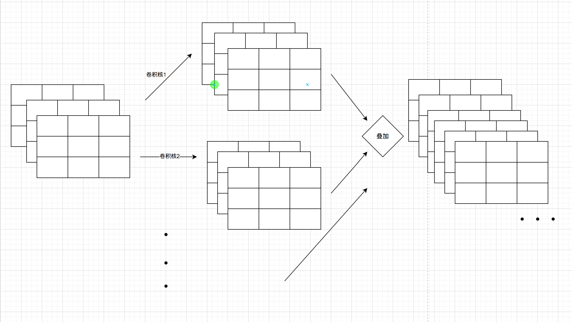
（1）卷积层主要通过提高维度（提高图像维度，例如黑白图像原本只有一维，RGB图像输入只有三维，通过卷积可以指定输出维度来提高维度以寻找特征），可以这样理解，维度就代表信息，比如黑白图像只有黑白信息，而RGB图像有三种颜色的信息，普通的卷积层（有些1x1的卷积是降维的，主要是为了减少运算量）主要就是提高通道数量来获取图像的特征，总而言之，卷积层就是用来提取图像位置特征的

这里可以看下RGB图像（三维）进行卷积层提高维度的过程

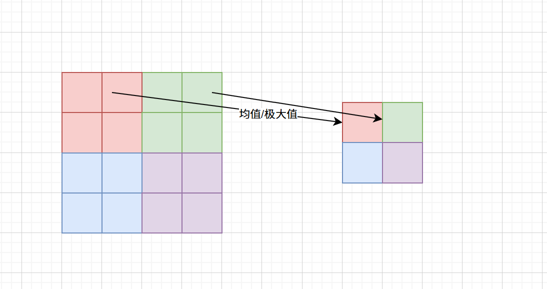
（2）池化层主要是通过对图像区域内求均值或极大值来缩小图像的像素点数，主要目的是图像的像素大小，主要目的是为了在后续池化层能够在一个更加全局的范围下寻找图像特征，或者有些池化层通过改变步数和填充值并不改变图像像素的大小，这是为了滤波或者其他目的，池化层改变最终输出的图像改变了像素大小，但并不改变训练中图像的维度，总而言之，池化层就是改变图像像素的多少，进而让图像的信息更加浓缩，让后面能够提取到更加全局的信息；

这里有个问题，为什么获取更大范围的信息不使用更大的卷积核而是使用池化层缩小图像像素呢？可以找下资料对比两种方式的优劣；

池化层示意图如图：

（2）普通的cnn神经网络

（1）构建卷积神经网络

有了卷积层核池化层，就可以着手构建卷积神经网络了，神经网络就是先让图像经过一些卷积层提取图像特征，然后再通过池化层去缩小图像，然后又重复通过卷积层、池化层，最后将所有得到的特征通过线性层去映射到目标上；

这里使用的模型是手写数字识别模型，也就是输入是一维的黑白图像，模型应该让黑白图像通过卷积层提高维度，再通过池化层减少图像像素，然后重复，最后通过线性层将所有特征通过学习的系数映射成十维的结果，也就是0-9；

构建一个简单的cnn卷积神经网络如下：

class conv_model(nn.Module):
    def __init__(self):
        super(conv_model, self).__init__()
        self.conv1 = nn.Conv2d(1, 32, kernel_size=3, padding=1)
        self.pool1 = nn.MaxPool2d(2, 2)
        self.conv2 = nn.Conv2d(32, 64, kernel_size=3, padding=1)
        self.pool2 = nn.MaxPool2d(2, 2)
        self.conv3 = nn.Conv2d(64, 128, kernel_size=3, padding=1)
        self.linear_1 = nn.Linear(128*7*7, 2048)
        self.linear_2 = nn.Linear(2048, 512)
        self.linear_3 = nn.Linear(512, 128)
        self.linear_4 = nn.Linear(128, 10)

    def forward(self, x):
        x = F.relu(self.conv1(x))
        x = self.pool1(x)
        x = F.relu(self.conv2(x))
        x = self.pool2(x)
        x = F.relu(self.conv3(x))
        x = x.view(-1, 128*7*7)
        x = F.relu(self.linear_1(x))
        x = F.relu(self.linear_2(x))
        x = F.relu(self.linear_3(x))
        y = F.softmax(self.linear_4(x), dim=1)
        return y

可以看到，这个模型先让图像通过一个卷积层从1通道到32通道，这里nn.Conv2d中参数kernel_size指定卷积核大小，padding指定在边缘进行多少像素填充，多少像素填充主要是看卷积核的，这里指定卷积核大小为3，因此进行1像素填充，如果是5，那就应该填充2，这样才能保证图像经过卷积层后图像通道变化，但图像像素不发生变化；

经过卷积层后让图像经过池化层，这里有两个参数，第一个参数指定池化核的大小，如果是一个数字就为矩形，元组则为长方形，第二个参数是池化的步长，这里选择核的大小为2，步长也是2，就像示意图一样，通过池化层后图像的像素点会减半；

同时卷积层和池化层都是线性的，要引入非线性才能更好地拟合，这里想线性神经网络一样，在使用卷积层和线性层后需要使用激活函数F.relu，这样引入非线性变换；

最后通过线性层给每个特征分配一个系数，将所有特征映射到结果中，在最后使用F.softmax将结果变为概率值，这核前面模型基本一样；

（2）训练和测试

训练模型和前面基本相同，获取数据，随机分类，前馈预测，结果进行反馈，更新参数

获取数据函数：

def get_data():
    transform = transforms.Compose([
        transforms.ToTensor(),
        transforms.Normalize((0.1307,), (0.3081,))
    ])
    train_data = datasets.MNIST(root="./data", train=True, download=False, transform=transform) # 获取训练数据
    test_data = datasets.MNIST(root="./data", train=False, download=False, transform=transform) # 获取测试数据
    train_data_loader = DataLoader(train_data, batch_size=64, shuffle=True) # 训练数据分类加载器
    test_data_loader = DataLoader(test_data, batch_size=64, shuffle=True)   # 测试数据加载器
    return train_data_loader, test_data_loader

训练模型：

def train_model(model, criterion, optimizer, train_data_loader):
    model.train()
    for step, [data, target] in enumerate(train_data_loader):   # 每轮训练64张图像
        target_pre = model(data)
        loss = criterion(target_pre, target)    # 计算损失
        optimizer.zero_grad()   # 清空梯度
        loss.backward() # 反向传播，通过计算参数的梯度，优化参数
        optimizer.step()    # 更新参数

测试模型：

def test_model(model, test_data_loader):
    model.eval()
    success_cnt = 0 # 成功数量
    test_total = 0  # 测试总数
    with torch.no_grad():
        for step, [data, target] in enumerate(test_data_loader):
            target_pre = model(data)
            if step == len(test_data_loader) - 1:   # 最后一个打印一下
                print(torch.argmax(target_pre, dim=1), target)
            success_cnt += (torch.argmax(target_pre, dim=1) == target).sum().item()
            test_total += len(data)
    return success_cnt / test_total # 返回成功率

主函数：

model = conv_model()    # 构造卷积神经网络
train_data_loader, test_data_loader = get_data()    # 获取训练构造数据和测试构造数据
train_time = 20 # 训练20次
success_list = [0.0 for i in range(train_time)] # 记录每次训练的成功率

criterion = nn.CrossEntropyLoss()   # 构造交叉熵损失函数
optimizer = optim.SGD(model.parameters(), lr=0.01)  # 构造优化器
for i in range(train_time):
    train_model(model, criterion, optimizer, train_data_loader)
    success_list[i] = test_model(model, test_data_loader)

print(success_list)
# 绘制成功率曲线
fig, axs = plt.subplots(1, 1)
axs.plot(success_list)

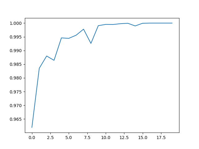
plt.show()

最终测试曲线和测试成功率如下：

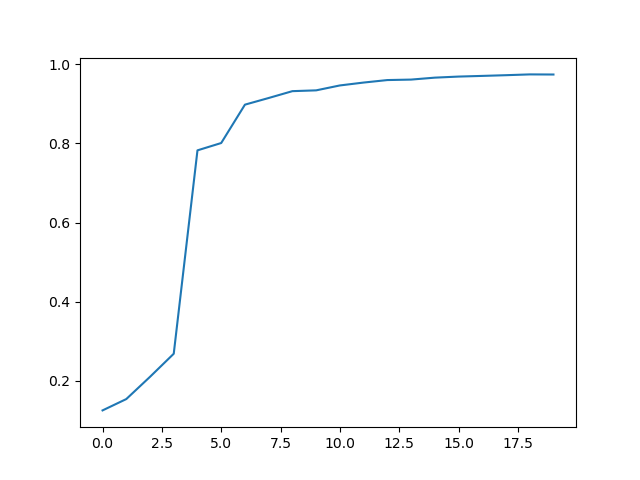
可以看到，这里训练后最后成功率也才稳定到0.97，这个成功率并不高，甚至不如线性模型，但是这个只是最简单的卷积神经网络，下面可以对卷积神经网络进行升级，最后成功率可以达到0.99，这就是inception cnn module

（2）inception模型

在构建cnn卷积神经网络模型时，有一个很关键的变量，那就是参数的选择，比如卷积核大小kernel_size，inception的核心思想是选取不同的kernel_size一起进行预测，通过训练来测试不同核对结果的效果，最终寻找不同核的影响系数，帮助我们进行一个最优化选择；

（1）构造inception层

这里构造一个inception_module，通过这个模型就是通过不同的卷积核：

class inception_model(nn.Module):
    def __init__(self, input_channel):
        super(inception_model, self).__init__()
        self.branch_1x1 = nn.Sequential(    # 1x1卷积，输出16通道
            nn.Conv2d(input_channel, 16, kernel_size=1, bias=False),
            nn.BatchNorm2d(16),
            nn.ReLU(inplace=True)
        )
        self.branch_3x3 = nn.Sequential(    # 3x3卷积，输出24通道
            nn.Conv2d(input_channel, 16, kernel_size=1, bias=False),
            nn.BatchNorm2d(16),
            nn.ReLU(inplace=True),
            nn.Conv2d(16, 24, kernel_size=3, padding=1, bias=False),
            nn.BatchNorm2d(24),
            nn.ReLU(inplace=True)
        )
        self.branch_5x5 = nn.Sequential(    # 5x5卷积，输出32通道
            nn.Conv2d(input_channel, 16, kernel_size=1, bias=False),    # 瓶颈层，主要目的是降维，减少通道
            nn.BatchNorm2d(16),
            nn.ReLU(inplace=True),
            nn.Conv2d(16, 32, kernel_size=5, padding=2, bias=False),
            nn.BatchNorm2d(32),
            nn.ReLU(inplace=True)
        )
        self.branch_p1x1 = nn.Sequential(   # 1x1卷积，输出32通道
            nn.MaxPool2d(3, 1, padding=1),
            nn.Conv2d(input_channel, 32, kernel_size=1, bias=False),
            nn.BatchNorm2d(32),
            nn.ReLU(inplace=True)
        )

    def forward(self, x):
        branch_1x1 = self.branch_1x1(x) # 通过1x1卷积层，输出16通道
        branch_3x3 = self.branch_3x3(x) # 通过3x3卷积层，输出24通道
        branch_5x5 = self.branch_5x5(x) # 通过5x5卷积层，输出32通道
        branch_p1x1 = self.branch_p1x1(x)   # 通过1x1卷积层，输出32通道
        return torch.cat([branch_1x1, branch_3x3, branch_5x5, branch_p1x1], 1) # output channel = 16+24+32+32

这里有四个通道，第一个通过的是16个不同的1x1的卷积核，第二个通过的是24个不同的3x3的卷积核，第三个是32个不同的5x5的卷积核，第四个是32个不同的1x1的卷积核；

这里nn.Sequential就是构造一个盒子，最终数据通过这个盒子依次将数据通过里面的所有层，相当于16+24+32+32；

最终torch.cat是将不同的通道层数进行拼接，这里输出的通道是所有网络输出的层数之和；

（2）cnn网络中引入inception层

构建inception层后，可以在cnn网络中加入inception层，通过测试不同卷积核大小来让模型更加拟合；

比如下面构建的cnn神经网络模型时，首先通过一个卷积层，从1通道通过3x3卷积核到32通道，然后通过2x2池化层减少图像的像素，然后就是通过自己构造的inception_model层了，这一层通过不同的卷积核输出指定的104通道数据，最后104通道实在太大了，通过卷积层进行降维，再通过池化层后再通过一次自己定义的嵌入层inception，最后通过线性层映射到结果上

class cnn_inception_model(nn.Module):
    def __init__(self):
        super(cnn_inception_model, self).__init__()
        self.conv1 = nn.Conv2d(1, 32, kernel_size=3, padding=1)
        self.pool1 = nn.MaxPool2d(2, 2)
        self.inception_model_1 = inception_model(32)

        self.conv2 = nn.Conv2d(104, 64, kernel_size=3, padding=1)
        self.pool2 = nn.MaxPool2d(2, 2)
        self.inception_model_2 = inception_model(64)

        self.conv3 = nn.Conv2d(104, 128, kernel_size=5, padding=2)

        self.linear = nn.Linear(128*7*7, 10)

    def forward(self, x):
        x = F.relu(self.conv1(x))
        x = self.pool1(x)
        x = self.inception_model_1(x)

        x = F.relu(self.conv2(x))
        x = self.pool2(x)
        x = self.inception_model_2(x)

        x = F.relu(self.conv3(x))

        x = x.view(-1, 128*7*7)
        y = F.softmax(self.linear(x), dim=1)
        return y

通过嵌入层能够取得很好的结果，届时测试的成功率可以达到0.99以上

（3）训练和测试模型

获取数据、训练数据和测试数据和普通cnn一样

def get_data():
    transform = transforms.Compose([
        transforms.ToTensor(),
        transforms.Normalize((0.1307, ), (0.3081, ))
    ])
    train_data = datasets.MNIST(root="./data", train=True, download=False, transform=transform)
    test_data = datasets.MNIST(root="./data", train=False, download=False, transform=transform)
    train_data_loader = DataLoader(train_data, batch_size=64, shuffle=True)
    test_data_loader = DataLoader(test_data, batch_size=64, shuffle=True)
    return train_data_loader, test_data_loader

def train_model(model, criterion, optimizer, train_data_loader):
    model.train()
    for step, [data, target] in enumerate(train_data_loader):
        target_pre = model(data)
        loss = criterion(target_pre, target)
        optimizer.zero_grad()
        loss.backward()
        optimizer.step()

def test_model(model, test_data_loader):
    model.eval()
    with torch.no_grad():
        success_cnt = 0
        total_cnt = 0
        for step, [data, target] in enumerate(test_data_loader):
            target_pre = model(data)
            success_cnt += (torch.argmax(target_pre, dim=1) == target).sum().item()
            total_cnt += len(data)
            if step == len(test_data_loader) - 1:
                print(torch.argmax(target_pre, dim=1), target)
        return success_cnt / total_cnt


train_data_loader, test_data_loader = get_data()
model = cnn_inception_model()
criterption = nn.CrossEntropyLoss()
optimizer = optim.SGD(model.parameters(), lr=0.01)

train_time = 20
success_list = [0.0 for i in range(train_time)]
for i in range(train_time):
    train_model(model, criterption, optimizer, train_data_loader)
    success_list[i] = test_model(model, test_data_loader)

print(success_list)
fig, axs = plt.subplots(1, 1)
axs.plot(success_list)

plt.show()

最终测试结果

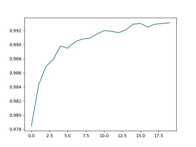
可以看到最后正确率稳定在0.99以上，通过增加一个inception层可以很好提高模型预测的成功率；

除此之外，卷积神经网络还有一个问题，就是卷积层度深度过大训练的结果反而不如浅层卷积层训练出来的模型，这是由于在进行反向传播时梯度会衰减，这里就需要引入cnn的另一个模型residual_model残差块；

（3）residual残差模型

残差模型的目的就是解决卷积层深度过大在训练时会出现梯度消失的问题，而解决方法是让原来的数据跳过中间几层直接加到后面的层中，最终函数为F(x) = H(x) + x，这样求梯度时x部分为1，可以有效缓解梯度消失问题

使用流程图表示为：

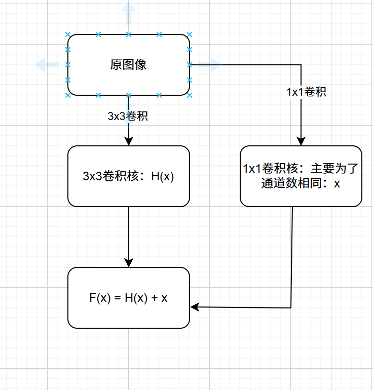
（1）残差块构建

残差块构建的时候需要注意F(x) = H(x) + x 的通道匹配，由于经过残差块后一般都要改变输出通道，因此我们需要通过卷积核为1的卷积层将输入直接扩展到输出通道再和进入卷积层的输出进行叠加

class residual_block(nn.Module):
    def __init__(self, input_channel, output_channle):
        super(residual_block, self).__init__()
        tem_channel = input_channel*2//3
        self.conv_1 = nn.Conv2d(input_channel, tem_channel, kernel_size=5, padding=2, bias=False)
        self.batch_normal1 = nn.BatchNorm2d(tem_channel)
        self.conv_2 = nn.Conv2d(tem_channel, output_channle, kernel_size=5, padding=2, bias=False)
        self.batch_normal2 = nn.BatchNorm2d(output_channle)

        self.conv_x = nn.Conv2d(input_channel, output_channle, kernel_size=1)
        self.batch_normalx = nn.BatchNorm2d(output_channle)
    def forward(self, x):
        y = self.batch_normal1(self.conv_1(x))
        y = F.relu(y)
        y = self.batch_normal2(self.conv_2(y))
        y = F.relu(y)
        x = self.conv_x(x)
        x = self.batch_normalx(x)
        z = F.relu(x + y)
        return z

（2）使用残差块构建cnn卷积神经网络

在神经网络中使用残差块代替卷积层构建可以让神经网络的层数达到更多，进而识别出图像的更多特征，这里使用两层卷积层、五层残差块进行神经网络的搭建

class cnn_des_module(nn.Module):
    def __init__(self):
        super(cnn_des_module, self).__init__()
        # 两层卷积层，五层残差层，最终通道数为1024通道
        self.conv1 = nn.Conv2d(1, 16, kernel_size=5, padding=2)
        self.conv2 = nn.Conv2d(16, 32, kernel_size=5, padding=2)
        
        self.res_module1 = residual_block(32, 64)
        self.res_module2 = residual_block(64, 128)
        self.pool1 = nn.MaxPool2d(2, 2)
        
        self.res_module3 = residual_block(128, 256)
        self.res_module4 = residual_block(256, 512)
        self.pool2 = nn.MaxPool2d(2, 2)
        self.res_module5 = residual_block(512, 1024)
        self.linear = nn.Linear(1024*7*7, 10)

    def forward(self, x):
        x = F.relu(self.conv1(x))
        x = F.relu(self.conv2(x))
        
        x = self.res_module1(x)
        x = self.res_module2(x)
        x = self.pool1(x)
        
        x = self.res_module3(x)
        x = self.res_module4(x)
        x = self.pool2(x)
        
        x = self.res_module5(x)
        x = x.view(-1, 1024*7*7)
        y = F.softmax(self.linear(x), dim=1)
        return y

（3）训练和测试

由于神经网络层数过多，所以可能存在训练时间过长的问题，这里也没有对训练进行什么加速，但是最后训练的准确度相比于前两个训练结果还是有一定的提升的；

值得注意的是，这个模型的训练时间很长，尽量在训练后保存模型参数，避免多次训练浪费时间

def get_data():
    transform = transforms.Compose([
        transforms.ToTensor(),
        transforms.Normalize((0.1307, ), (0.3081, ))
    ])

    train_data = datasets.MNIST(root="./data", train=True, download=False, transform=transform)
    test_data = datasets.MNIST(root="./data", train=True, download=False, transform=transform)
    train_data_loader = DataLoader(train_data, batch_size=64, shuffle=True)
    test_data_loader = DataLoader(test_data, batch_size=64, shuffle=True)
    return train_data_loader, test_data_loader

def train_module(model, criterion, optimizer, train_data_loader):
    model.train()
    for step, [data, target] in enumerate(train_data_loader):
        target_predict = model(data)
        loss = criterion(target_predict, target)
        optimizer.zero_grad()
        loss.backward()
        optimizer.step()

def test_module(model, test_data_loader):
    model.eval()
    success_num = 0
    total_num = 0
    with torch.no_grad():
        for step, [data, target] in enumerate(test_data_loader):
            target_predict = model(data)
            success_num += (torch.argmax(target_predict, dim=1) == target).sum().item()
            total_num += len(data)
            if step == 0:
                print(torch.argmax(target_predict, dim=1), target)
    return success_num / total_num

train_data_loader, test_data_loader = get_data()
model = cnn_des_module()
criterion = nn.CrossEntropyLoss()
optimizer = optim.SGD(model.parameters(), lr=0.01)

train_time = 20
success_list = [0.0 for i in range(train_time)]
for i in range(train_time):
    train_module(model, criterion, optimizer, train_data_loader)
    success_list[i] = test_module(model, test_data_loader)
    print(success_list[i])

print(success_list)
torch.save(model.state_dict(), "cnn_residual_module.pth")   # 保存模型参数
fig, axs = plt.subplots(1, 1)
axs.plot(success_list)

plt.show()

这里测试和训练和之前的完全一样，直接看结果

最终达到了100%

（4）保存模型并使用模型进行预测

（1）保存模型

上述模型在进行训练完成后可以进行保存，这样下次就可以直接使用了，保存分为两种方式；

一种是只保存状态字典，简单来说就是只保存学习参数（权重和偏置），但是在使用中需要先导入模型的类结构，再在类结构上导入模型的学习参数；

另一种是保存整个模型，这样在使用中不需要先引入模型类，直接使用即可，但是内存会增加；

这里使用保存状态字典的方式进行保存，具体操作是在模型训练完后调用torch.save函数传入训练完的模型和保存的名称，如下：

torch.save(model.state_dict(), "cnn_inception_module.pth")

如果保存整个模型则第一个参数直接传递模型即可，如下：

torch.save(model, "cnn_inception_module.pth")

（2）加载模型并进行推演

如果使用保存模型的方法是直接保存整个模型，那么就不用搭建神经网络模型，直接使用加载就行，如果使用保存状态字典的方式进行保存，那么就要先写出模型结构再引入模型参数，至于模型结构就是上面构建模型的类

先实例化一个神经网络类，再在神经网络类中加载状态字典

cnn_inception_module = cnn_inception_model()    # 实例化
cnn_inception_module.load_state_dict(torch.load("cnn_inception_module.pth", map_location="cpu"))    # 加载状态字典

这里我将所有训练都封装成了一个类，这个推演的设计十分灵活，主要注意的事情只有一点，那就是推演的图像必须和训练时的图像相似，否则效果非常差

比如这里训练的是一个28*28原始数据集合，如果你使用一个任意宽高的图像进行直接压缩成28*28的图像，那么推演的正确率将不堪入目，这是因为原始手写数据集合是非常标准的数字处于图像中间的集合，所以我们最好的方法是使用正方形的图像进行推演，这样正确率还是能够在0.9以上，如果缺失没有正方形图像，也可以对图像进行一些预处理达到比较高的正确率，这里准备了一个标准的正方形图像和任意尺寸图像进行推演

正方形图像可以直接进行压缩，不用考虑数字会变扁变瘦的问题，但是任意尺寸大小的图像就要考虑裁剪的问题，预处理函数如下

正方形图像直接压缩

    def img_change(self, img_road, target_size=(28, 28)):
        # 将比例放大成正方形
        img = Image.open(img_road).convert("L")
        img = img.resize(target_size)
        return img

任意比例图像要经过处理

    def img_complicate_change(self, img_name, target_size=(28, 28), resize_size=(21, 21)):
        img = cv2.imread(img_name, cv2.IMREAD_GRAYSCALE)    # 以灰度方式读取图像
        img_blurred = cv2.GaussianBlur(img, (5, 5), 0)  # 进行高斯滤波
        _, img_binary = cv2.threshold(img_blurred, np.mean(img_blurred)+10, 255, cv2.THRESH_BINARY) # 二值化

        contours, _ = cv2.findContours(img_binary, cv2.RETR_EXTERNAL, cv2.CHAIN_APPROX_SIMPLE)  # 获取轮廓
        largest_contour = max(contours, key=cv2.contourArea)    # 获取最大轮廓
        x, y, w, h = cv2.boundingRect(largest_contour)  # 获取边界框
        fig_img = img_binary[y:y+h, x:x+w]  # 获取最大轮廓的图像


        scale = min(resize_size[0] / w, resize_size[1] / h) # 计算缩放比例
        resized_w, resized_h = int(w * scale + 1), int(h * scale + 1)   # 计算缩放后的大小
        resized_img = cv2.resize(fig_img, (resized_w, resized_h), interpolation=cv2.INTER_AREA) # 缩放图像
        final_img = np.zeros(target_size, dtype=np.uint8)   # 创建目标图像
        paste_x, paste_y = (target_size[0] - resized_w) // 2, (target_size[1] - resized_h) // 2 # 计算粘贴位置
        final_img[paste_y:paste_y+resized_h, paste_x:paste_x+resized_w] = resized_img   # 粘贴图像
        pil_img = Image.fromarray(final_img, mode="L")  # 转换为PIL图像

        return pil_img

同时不要忘记我们在读取原始手写数据时候进行的预处理，这里自己写的数字一样要通过这些处理，否则效果很差

    transform = transforms.Compose([
        transforms.ToTensor(),
        transforms.Normalize((0.1307, ), (0.3081, ))
    ])    # 原始数据的预处理
    train_data = datasets.MNIST(root="./data", train=True, download=False, transform=transform)
    test_data = datasets.MNIST(root="./data", train=False, download=False, transform=transform)

自己写的也要进行一样的处理

    transform = transforms.Compose([
        transforms.ToTensor(),
        transforms.Normalize((0.1307, ), (0.3081, ))
    ])

同时我将所有训练都封装成了一个类

class inception_predict_model():
    def __init__(self, inception_module, test_filename, module_path):
        self.module = inception_module
        self.test_filename = test_filename
        self.module.load_state_dict(torch.load(module_path, map_location=torch.device('cpu')))
        self.module.eval()    # 测试模式
        self.fig, self.axs = plt.subplots(10, 10, figsize=(10, 10))
        self.success_cnt = 0

    def predict(self):
        for i in range(10):
            for j in range(10):
                if self.test_filename == "hand_image":  # 这里存放的是任意比例的图像
                    img = self.img_complicate_change(f"{self.test_filename}/{i}/{j}.png") # 图像读取并裁剪
                else:   # 这个是正方形比例的图像
                    img = self.img_change(f"{self.test_filename}/{i}/{j}.png")
                transform = torchvision.transforms.Compose(
                    [torchvision.transforms.ToTensor(),
                     transforms.Normalize((0.1307, ), (0.3081, ))]
                )
                img = transform(img)    # 转换为张量，并作同样的归一化
                img = torch.reshape(img, (1, 1, 28, 28))    # 改变张量的维度
                with torch.no_grad():
                    predict_result = self.module(img)   # 预测结果
                    print(f"{i}, {j}", end=" ")
                    print(predict_result)
                self.axs[i][j].imshow(img.squeeze(), cmap="gray")   # plt 显示是否正确
                self.axs[i][j].axis("off")
                if predict_result.argmax(1)[0] == i:
                    self.success_cnt += 1
                    self.axs[i][j].set_title(f"{predict_result.argmax(1)[0]}", color="green", fontsize=8)
                else:
                    self.axs[i][j].set_title(f"{predict_result.argmax(1)[0]}", color="red", fontsize=8)
    def img_change(self, img_road, target_size=(28, 28)):
        # 将比例放大成正方形
        img = Image.open(img_road).convert("L")
        img = img.resize(target_size)
        return img

    def img_complicate_change(self, img_name, target_size=(28, 28), resize_size=(21, 21)):
        img = cv2.imread(img_name, cv2.IMREAD_GRAYSCALE)    # 以灰度方式读取图像
        img_blurred = cv2.GaussianBlur(img, (5, 5), 0)  # 进行高斯滤波
        _, img_binary = cv2.threshold(img_blurred, np.mean(img_blurred)+10, 255, cv2.THRESH_BINARY) # 二值化

        contours, _ = cv2.findContours(img_binary, cv2.RETR_EXTERNAL, cv2.CHAIN_APPROX_SIMPLE)  # 获取轮廓
        largest_contour = max(contours, key=cv2.contourArea)    # 获取最大轮廓
        x, y, w, h = cv2.boundingRect(largest_contour)  # 获取边界框
        fig_img = img_binary[y:y+h, x:x+w]  # 获取最大轮廓的图像


        scale = min(resize_size[0] / w, resize_size[1] / h) # 计算缩放比例
        resized_w, resized_h = int(w * scale + 1), int(h * scale + 1)   # 计算缩放后的大小
        resized_img = cv2.resize(fig_img, (resized_w, resized_h), interpolation=cv2.INTER_AREA) # 缩放图像
        final_img = np.zeros(target_size, dtype=np.uint8)   # 创建目标图像
        paste_x, paste_y = (target_size[0] - resized_w) // 2, (target_size[1] - resized_h) // 2 # 计算粘贴位置
        final_img[paste_y:paste_y+resized_h, paste_x:paste_x+resized_w] = resized_img   # 粘贴图像
        pil_img = Image.fromarray(final_img, mode="L")  # 转换为PIL图像

        return pil_img
    
    def show_result(self):
        print(f"success probability: {self.success_cnt / 100}")
        plt.tight_layout()  # 调整子图之间的间距
        plt.show()

这里有些参数设置很随机，比如裁剪的图像大小相差1像素可能正确率会下降5%（如果考虑原图只有28像素也正常），可以参照一下原始数据集来参考一下自己的应该怎么变得和原始图像一样的格式；

这里放一下原始的手写数据训练集合，获取代码如下，这里get_data函数用到了上面的

# train_data_loader, test_data_loader = get_data()
# fig, axs = plt.subplots(5, 5, figsize=(10, 10))
# for i in range(5):
#     for j in range(5):
#         images, labels = next(iter(train_data_loader))
#         img = images[0]
#         label = labels[0]
#         img = np.array(img[0])
#         axs[i][j].imshow(img, cmap="gray")
#
# plt.show()

最终显示25个图像如下

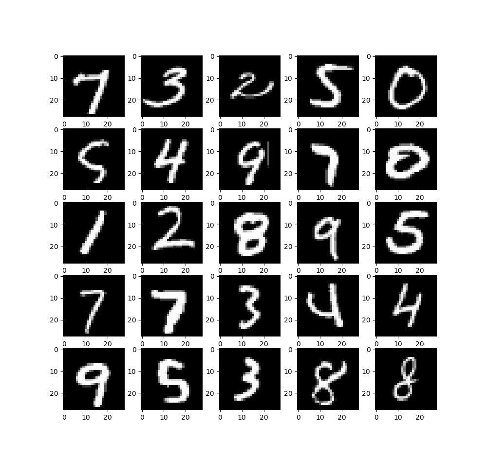
一般就是居中处理一下就行了，上面也就是用到了滤波和数字居中处理

一下推理均使用inception模型进行推理，有一组数据在绘制时候是在正方形画板上绘制的，一组是在任意比例的画板上绘制的

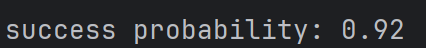
使用正方形图像推理的准确度较高，达到0.92

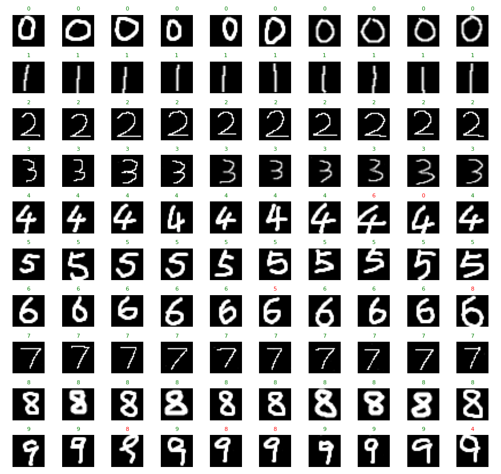
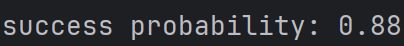
使用任意比例的图像推理就一般，只有0.88

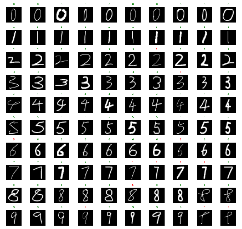
因为这里显示的图像是处理过的，没有看出任意比例，但是原始图像是任意采集的

这里推理明显没有训练的准确率那么高，个人理解是绘制图像像素多，训练图像的像素很少，进行压缩后导致一些信息丢失，应该不是过拟合的问题，对于这个问题，我暂时还没有找到比较理想的解决方案

（5）结束

本文章有大量个人理解，如有错误，还望指出