前言
在上文《pytorch线性回归》一文中,我们有如下线性回归训练代码:
python
def train(inputs, target, w, times=50, step=0.01):
    global loss, output
    for i in range(times):
        output = inputs.mv(w)
        loss = (output - target).pow(2).sum()

        loss.backward()

        w.data -= step * w.grad
        w.grad.zero_()

    #...
其中:
- output = inputs.mv(w):输入矩阵与权重向量相乘,也就是前向传播过程。
- loss = (output - target).pow(2).sum():计算损失值,即 ∑ ∣ Y − X ∣ 2 \sum|Y-X|^2 ∑∣Y−X∣2。也可以用均方差 1 n ∑ ∣ Y − X ∣ 2 \frac{1}{n}\sum|Y-X|^2 n1∑∣Y−X∣2,实质上应该不影响结果。
- loss.backward():反向传播,计算叶子节点偏导。
- w.data -= step * w.grad:梯度下降迭代过程,对权重向量进行更新。
- w.grad.zero_():清空权重向量的grad值,防止梯度累积影响后续训练过程。这一步与上一步的梯度下降迭代一起称为优化过程。
其实pytorch中已经有了相关损失函数、线性计算、优化过程的函数,下面看看如何基于pytorch这些函数来做线性回归的训练。
1、导入相关库
python
import torch
import matplotlib.pyplot as plt

from torch import nn, optim
from time import perf_counter
导入如上库,其中:
- torch:pytorch库
- matplotlib.pyplot:数据图形绘制库
- torch下的nn和optim:nn是Neural Network的缩写,optim则是优化器相关
- time下的perf_counter用于计算训练耗时
2、准备数据
用之前生成的数据,其中y是用y = 1.2 * x + 3 + 0.2 * torch.rand(x.size())生成的,即 y ≈ 1.2 x + 3 y \approx 1.2x + 3 y≈1.2x+3。并且通过view函数把一行50列的数据转换成50行一列的数据,方便后续计算:
python
x = torch.Tensor(
    [-5.0000, -4.7959, -4.5918, -4.3878, -4.1837, -3.9796, -3.7755, -3.5714, -3.3673, -3.1633, -2.9592, -2.7551,
     -2.5510, -2.3469, -2.1429, -1.9388, -1.7347, -1.5306, -1.3265, -1.1224, -0.9184, -0.7143, -0.5102, -0.3061,
     -0.1020, 0.1020, 0.3061, 0.5102, 0.7143, 0.9184, 1.1224, 1.3265, 1.5306, 1.7347, 1.9388, 2.1429, 2.3469, 2.5510,
     2.7551, 2.9592, 3.1633, 3.3673, 3.5714, 3.7755, 3.9796, 4.1837, 4.3878, 4.5918, 4.7959, 5.0000])
y = torch.Tensor(
    [-2.9354, -2.6106, -2.5070, -2.1573, -2.0062, -1.7503, -1.3872, -1.2434, -1.0399, -0.7758, -0.3666, -0.2873,
     -0.0095, 0.3227, 0.4873, 0.8658, 1.0763, 1.2531, 1.4564, 1.7801, 2.0736, 2.1845, 2.4290, 2.6380, 2.9424, 3.3018,
     3.3983, 3.6191, 4.0433, 4.1419, 4.5190, 4.7428, 4.9229, 5.1000, 5.4449, 5.7140, 5.8567, 6.1416, 6.3126, 6.6015,
     6.9624, 7.1786, 7.4084, 7.5916, 7.9413, 8.1177, 8.4207, 8.5427, 8.8767, 9.1533])

print(x.shape, y.shape)
# 输出torch.Size([50]) torch.Size([50])

x = x.view(-1, 1)
y = y.view(-1, 1)

print(x.shape, y.shape)
# 输出torch.Size([50, 1]) torch.Size([50, 1])
3、定义绘制数据图表函数
入参x、y是原始数据x、y;calcOutput是训练后根据x和模型权重计算的输出值;loss则是损失值:
python
def draw_result(x, y, calcOutput, loss):
    plt.scatter(x.numpy(), y.numpy())
    plt.plot(x.numpy(), calcOutput.data.numpy(), 'r-', lw=2)
    plt.text(0.5, 0, 'loss=%s' % loss.item())
    plt.show()
4、定义自己的模型
定义自己的线性回归模型类MyLinear,该类继承nn.Module。并且在该类的初始化函数__init__中定义linear,linear实际上是用nn中预设好的线性神经网络模块nn.linear来构造线性模型。nn.linear的in_features代表输入数据的维度,out_features则是代表输出参数的维度,我们这里的数据都是一维的,因此两个值都是1。
python
class MyLiner(nn.Module):
    def __init__(self):
        super(MyLiner, self).__init__()
        self.linear = nn.Linear(in_features=1, out_features=1)

    def forward(self, x):
        return self.linear(x)
5、定义训练函数
训练函数入参model就是我们的自定义模型实例;x、y是原始数据;times代表训练次数,默认5w次;lr(learning rate)代表学习率,也可以理解为步长,默认0.01。
函数里我们这里用nn预设值的均方差函数MSELoss(也就是前文提到的 1 n ∑ ∣ Y − X ∣ 2 \frac{1}{n}\sum|Y-X|^2 n1∑∣Y−X∣2)来作为损失函数,梯度下降则改为optim下的随机梯度下降算法SGD。随机梯度下降相比于普通梯度下降,一方面可以避免一次性加载全部数据导致内存溢出问题,有能防止优化的时候陷入局部最小值。
在梯度下降的for循环迭代中,则是先把x给自定义模型计算当前权重下的输出值output,再用 1 n ∑ ∣ Y − X ∣ 2 \frac{1}{n}\sum|Y-X|^2 n1∑∣Y−X∣2计算损失值。之后先把优化器optimizer的梯度清零防止累积影响后续训练,然后backward反向传播计算梯度,最后用step更新优化器的权重值。
训练后打印权重值model.parameters、损失值loss,并绘制数据图表
python
def train(model, x, y, times=50000, lr=1e-2):
    criterion = nn.MSELoss()
    optimizer = optim.SGD(model.parameters(), lr=lr)

    global loss, output
    for i in range(times):
        output = model(x)
        loss = criterion(output, y)

        optimizer.zero_grad()
        loss.backward()
        optimizer.step()

    print(list(model.parameters()))
    print(loss)

    draw_result(x, y, output, loss)
6、串联逻辑
把上面函数逻辑串联起来:
python
model = MyLinear()
start = perf_counter()
train(model, x, y)
end = perf_counter()
time = end - start
print("time: %s" % time)
7、整体代码
python
# my_linear.py
import torch
import matplotlib.pyplot as plt
from torch import nn, optim
from time import perf_counter
x = torch.Tensor(
[-5.0000, -4.7959, -4.5918, -4.3878, -4.1837, -3.9796, -3.7755, -3.5714, -3.3673, -3.1633, -2.9592, -2.7551,
-2.5510, -2.3469, -2.1429, -1.9388, -1.7347, -1.5306, -1.3265, -1.1224, -0.9184, -0.7143, -0.5102, -0.3061,
-0.1020, 0.1020, 0.3061, 0.5102, 0.7143, 0.9184, 1.1224, 1.3265, 1.5306, 1.7347, 1.9388, 2.1429, 2.3469, 2.5510,
2.7551, 2.9592, 3.1633, 3.3673, 3.5714, 3.7755, 3.9796, 4.1837, 4.3878, 4.5918, 4.7959, 5.0000])
y = torch.Tensor(
[-2.9354, -2.6106, -2.5070, -2.1573, -2.0062, -1.7503, -1.3872, -1.2434, -1.0399, -0.7758, -0.3666, -0.2873,
-0.0095, 0.3227, 0.4873, 0.8658, 1.0763, 1.2531, 1.4564, 1.7801, 2.0736, 2.1845, 2.4290, 2.6380, 2.9424, 3.3018,
3.3983, 3.6191, 4.0433, 4.1419, 4.5190, 4.7428, 4.9229, 5.1000, 5.4449, 5.7140, 5.8567, 6.1416, 6.3126, 6.6015,
6.9624, 7.1786, 7.4084, 7.5916, 7.9413, 8.1177, 8.4207, 8.5427, 8.8767, 9.1533])
print(x.shape, y.shape)
x = x.view(-1, 1)
y = y.view(-1, 1)
print(x.shape, y.shape)
def draw_result(x, y, calcOutput, loss):
# if torch.cuda.is_available():
# output = output.cpu()
plt.scatter(x.numpy(), y.numpy())
plt.plot(x.numpy(), calcOutput.data.numpy(), 'r-', lw=2)
plt.text(0.5, 0, 'loss=%s' % loss.item())
plt.show()
class MyLinear(nn.Module):
def __init__(self):
super(MyLinear, self).__init__()
self.linear = nn.Linear(in_features=1, out_features=1)
def forward(self, x):
return self.linear(x)
def train(model, x, y, times=50000, lr=1e-2):
criterion = nn.MSELoss()
optimizer = optim.SGD(model.parameters(), lr=lr)
global loss, output
for i in range(times):
output = model(x)
loss = criterion(output, y)
optimizer.zero_grad()
loss.backward()
optimizer.step()
print(list(model.parameters()))
print(loss)
draw_result(x, y, output, loss)
model = MyLinear()
start = perf_counter()
train(model, x, y)
end = perf_counter()
time = end - start
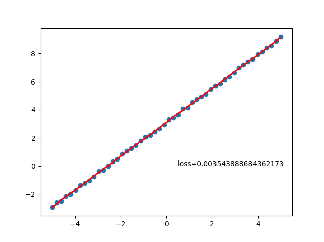
print("time: %s" % time)9、训练结果
执行python my_linear.py输出如下结果,可以看出训练出来损失值是0.0035,权重分别是1.2043和3.0897,和我们生成函数的1.2、3很接近,符合预期。
text
$ python my_linear.py
torch.Size([50]) torch.Size([50])
torch.Size([50, 1]) torch.Size([50, 1])
[Parameter containing:
tensor([[1.2043]], requires_grad=True), Parameter containing:
tensor([3.0897], requires_grad=True)]
tensor(0.0035, grad_fn=<MseLossBackward0>)
从数据图形也能看出训练模型基本拟合原始数据: