机器学习算法全景解析:从理论到实践
引言
机器学习作为人工智能的核心组成部分,正在深刻地改变我们的世界。从推荐系统到自动驾驶,从医疗诊断到金融风控,机器学习算法无处不在。本文将全面系统地介绍机器学习的主要算法类别及其核心知识点,帮助读者构建完整的机器学习知识体系。
一、机器学习基础概念
1.1 机器学习定义
机器学习是一门研究如何通过数据自动改进计算机程序性能的学科。其核心思想是:通过算法解析数据,从中学习规律,然后对真实世界中的事件做出决策或预测。
1.2 机器学习分类
-
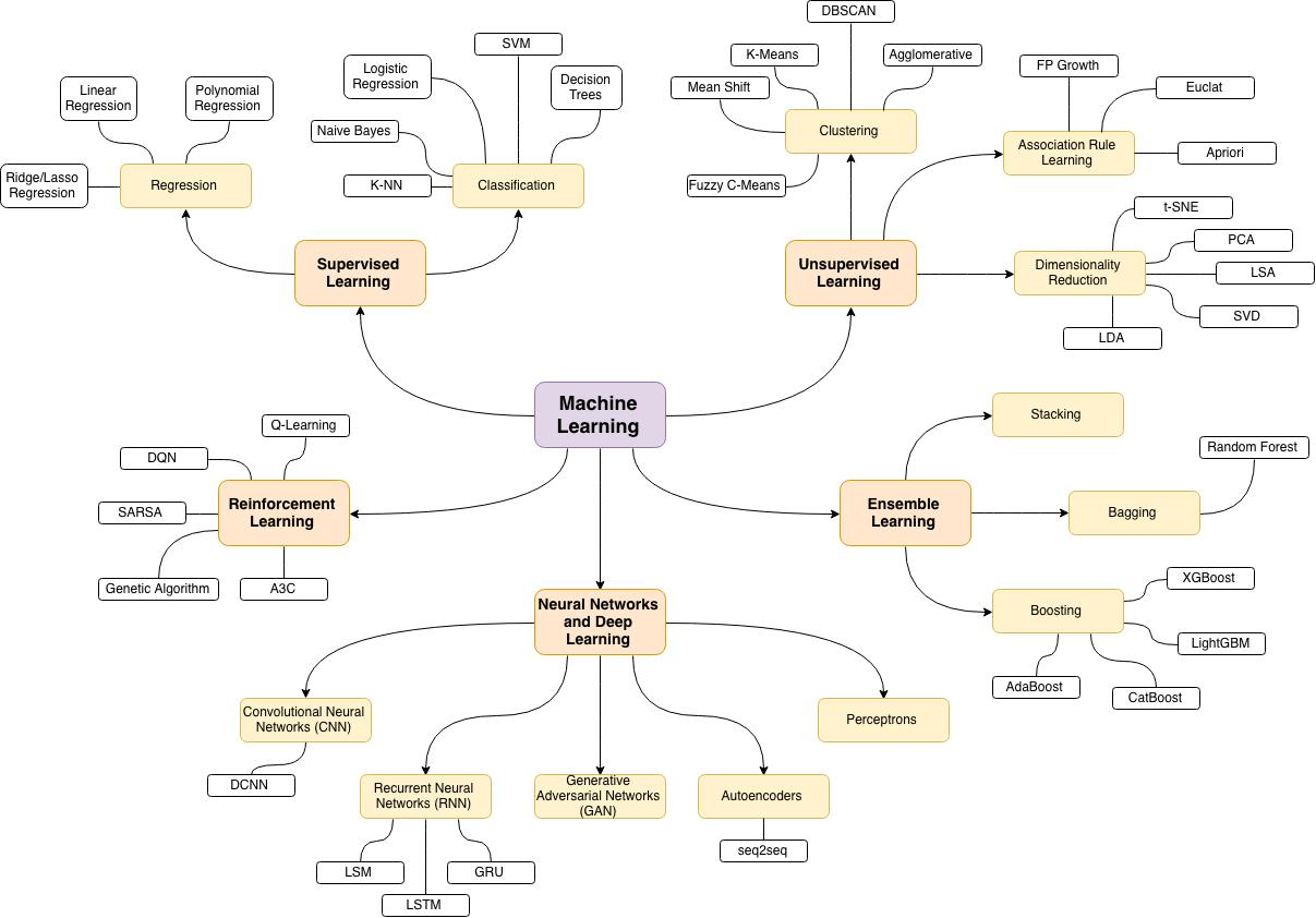
监督学习:使用带有标签的数据训练模型
-
无监督学习:使用无标签的数据发现内在模式
-
半监督学习:结合少量标注数据和大量未标注数据
-
强化学习:通过与环境交互学习最优策略
1.3 基本术语
-
特征(Feature):输入变量
-
标签(Label):输出变量(监督学习)
-
样本(Sample):单个数据点
-
数据集(Dataset):样本集合
-
训练(Training):模型学习过程
-
推理(Inference):模型预测过程
二、监督学习算法
2.1 线性回归
核心思想:建立特征与连续目标值之间的线性关系
数学模型 :
y = \\beta_0 + \\beta_1x_1 + \\beta_2x_2 + ... + \\beta_nx_n + \\epsilon
损失函数 :均方误差(MSE)
MSE = \\frac{1}{n}\\sum_{i=1}\^{n}(y_i - \\hat{y_i})\^2
优化方法:
-
最小二乘法(解析解)
-
梯度下降(数值解)
正则化变体:
-
岭回归(L2正则化)
-
Lasso回归(L1正则化)
-
ElasticNet(L1+L2正则化)
2.2 逻辑回归
核心思想:解决二分类问题,输出概率值
数学模型 :
P(y=1\|x) = \\frac{1}{1 + e\^{-(\\beta_0 + \\beta\^Tx)}}
损失函数 :交叉熵损失
J(\\theta) = -\\frac{1}{n}\\sum_{i=1}\^{n}\[y_i\\log(\\hat{y_i}) + (1-y_i)\\log(1-\\hat{y_i})\]
多分类扩展:
-
One-vs-Rest (OvR)
-
Softmax回归(多类逻辑回归)
2.3 支持向量机(SVM)
核心思想:寻找最大间隔超平面分离数据
线性可分情况 :
\\min_{w,b} \\frac{1}{2}\|\|w\|\|\^2 s.t. y_i(w\^Tx_i + b) \\geq 1
非线性扩展:
-
核技巧:将数据映射到高维空间
-
常用核函数:多项式核、高斯核(RBF)、Sigmoid核
软间隔SVM :处理噪声和不可分数据
\\min_{w,b,\\xi} \\frac{1}{2}\|\|w\|\|\^2 + C\\sum_{i=1}\^{n}\\xi_i
2.4 决策树
核心思想:基于特征对数据递归划分
分裂标准:
-
信息增益(ID3算法)
-
信息增益比(C4.5算法)
-
基尼指数(CART算法)
剪枝策略:
-
预剪枝:提前终止树生长
-
后剪枝:生成完整树后剪枝
优缺点:
-
优点:可解释性强、无需特征缩放、处理混合类型数据
-
缺点:容易过拟合、对数据微小变化敏感
2.5 随机森林
核心思想:集成多棵决策树,通过投票提高性能
关键机制:
-
Bagging:自助采样构建多个训练集
-
特征随机性:每个节点分裂时随机选择特征子集
超参数:
-
树的数量(n_estimators)
-
最大深度(max_depth)
-
最小分裂样本数(min_samples_split)
2.6 梯度提升机
核心思想:逐步添加弱学习器,纠正前一个模型的错误
常见实现:
-
XGBoost:添加正则化项,防止过拟合
-
LightGBM:基于直方图的优化,训练速度快
-
CatBoost:专门处理类别特征
核心公式 :
F_m(x) = F_{m-1}(x) + \\gamma_m h_m(x)
三、无监督学习算法
3.1 K均值聚类
核心思想:将数据划分为K个簇,使簇内方差最小
算法步骤:
-
随机选择K个初始质心
-
将每个点分配到最近的质心
-
重新计算质心位置
-
重复2-3步直到收敛
局限性:
-
需要预先指定K值
-
对初始质心敏感
-
只能发现球形簇
3.2 层次聚类
核心思想:通过层次分解或合并构建聚类树
两种策略:
-
凝聚式(自底向上):初始每个样本为一类,逐步合并
-
分裂式(自顶向下):初始所有样本为一类,逐步分裂
距离度量:
-
单链接:最小簇间距离
-
全链接:最大簇间距离
-
平均链接:平均簇间距离
3.3 主成分分析(PCA)
核心思想:通过正交变换将相关变量转为不相关的主成分
数学原理:
-
计算协方差矩阵
-
特征值分解
-
选择前k大特征值对应的特征向量
应用场景:
-
数据降维
-
数据可视化
-
噪声过滤
3.4 异常检测算法
隔离森林 :通过随机分割隔离异常点
One-Class SVM :学习正常数据的边界
自编码器:通过重建误差检测异常
四、神经网络与深度学习
4.1 感知机与多层感知机
单层感知机 :最简单的神经网络结构
y = f(\\sum_{i=1}\^{n}w_ix_i + b)
激活函数:
-
Sigmoid:\\sigma(x) = \\frac{1}{1 + e\^{-x}}
-
Tanh:\\tanh(x) = \\frac{e\^x - e\^{-x}}{e\^x + e\^{-x}}
-
ReLU:f(x) = \\max(0, x)
反向传播算法:通过链式法则计算梯度
4.2 卷积神经网络(CNN)
核心结构:
-
卷积层:提取局部特征
-
池化层:降维,保持平移不变性
-
全连接层:整合特征进行分类
经典架构:
-
LeNet-5:早期成功应用于手写数字识别
-
AlexNet:深度学习复兴的标志
-
ResNet:残差连接解决梯度消失
4.3 循环神经网络(RNN)
核心思想:处理序列数据,具有记忆功能
变体结构:
-
LSTM:门控机制解决长程依赖
-
GRU:简化版LSTM,计算效率更高
应用领域:
-
自然语言处理
-
时间序列预测
-
语音识别
4.4 Transformer与自注意力机制
自注意力机制:计算输入序列中每个位置与其他位置的相关性
Transformer架构:
-
编码器-解码器结构
-
多头注意力机制
-
位置编码
衍生模型:
-
BERT:双向编码器表示
-
GPT:生成式预训练变换器
五、模型评估与优化
5.1 评估指标
分类问题:
-
准确率、精确率、召回率、F1分数
-
ROC曲线与AUC值
-
混淆矩阵
回归问题:
-
均方误差(MSE)
-
平均绝对误差(MAE)
-
R平方系数
5.2 偏差-方差权衡
偏差 :模型预测值与真实值的差异
方差 :模型对训练数据变化的敏感性
权衡策略:通过正则化、集成学习等方法平衡
5.3 交叉验证
k折交叉验证 :将数据分为k份,轮流使用k-1份训练,1份测试
留一法交叉验证 :k等于样本数
分层交叉验证:保持每折中类别比例相同
5.4 超参数调优
网格搜索 :遍历所有参数组合
随机搜索 :随机采样参数空间
贝叶斯优化:基于先前评估结果选择下一个参数
六、实际应用考虑
6.1 特征工程
特征缩放 :标准化、归一化
特征编码 :独热编码、标签编码
特征选择 :过滤法、包装法、嵌入法
特征提取:PCA、LDA、t-SNE
6.2 类别不平衡处理
采样方法:
-
过采样(如SMOTE)
-
欠采样
算法层面:
-
类别权重调整
-
代价敏感学习
6.3 模型部署与监控
部署方式 :批量预测、实时推理
监控指标 :预测准确性、响应延迟、资源使用率
模型更新:全量更新、增量更新、在线学习
七、总结与展望
机器学习算法种类繁多,各有其适用场景和优缺点。在实际应用中,需要根据具体问题和数据特点选择合适的算法。未来机器学习的发展趋势包括:
-
自动化机器学习:减少人工干预
-
可解释AI:增强模型透明度
-
联邦学习:保护数据隐私
-
强化学习应用扩展:解决更复杂决策问题
掌握机器学习算法不仅需要理解数学原理,还需要通过实践积累经验。希望本文能为您的机器学习学习之旅提供有价值的参考。
进一步学习资源:
-
《机器学习》周志华
-
《Pattern Recognition and Machine Learning》Bishop
-
Coursera: Machine Learning by Andrew Ng
-
Kaggle竞赛:实践平台
注:本文仅概述了机器学习算法的主要知识点,每个算法都值得深入研究和实践。建议读者结合实际项目,深化对各类算法的理解。
写一篇关于机器学习各个算法的知识点的博客,要求内容详细,附有代码实例,不少于10000字
机器学习算法全景解析:从理论到实践
引言
机器学习作为人工智能的核心组成部分,正在深刻地改变我们的世界。从推荐系统到自动驾驶,从医疗诊断到金融风控,机器学习算法无处不在。本文将全面系统地介绍机器学习的主要算法类别及其核心知识点,通过详细的数学解释和完整的代码示例,帮助读者构建完整的机器学习知识体系。
一、机器学习基础概念
1.1 机器学习定义
机器学习是一门研究如何通过数据自动改进计算机程序性能的学科。其核心思想是:通过算法解析数据,从中学习规律,然后对真实世界中的事件做出决策或预测。
1.2 机器学习分类
-
监督学习:使用带有标签的数据训练模型,包括分类和回归问题
-
无监督学习:使用无标签的数据发现内在模式,包括聚类和降维
-
半监督学习:结合少量标注数据和大量未标注数据进行学习
-
强化学习:通过与环境交互学习最优策略,获得最大累积奖励
1.3 基本术语详解
-
特征(Feature):描述数据的输入变量,可以是数值型、类别型等
-
标签(Label):在监督学习中的输出变量,是我们要预测的目标
-
样本(Sample):单个数据实例,包含一组特征和可能的标签
-
数据集(Dataset):样本的集合,通常分为训练集、验证集和测试集
-
训练(Training):模型从数据中学习规律的过程
-
推理(Inference):使用训练好的模型对新数据进行预测
1.4 开发环境设置
在开始代码实践前,我们先设置开发环境:
python
# 导入必要的库
import numpy as np
import pandas as pd
import matplotlib.pyplot as plt
import seaborn as sns
from sklearn.model_selection import train_test_split, cross_val_score
from sklearn.metrics import accuracy_score, mean_squared_error, classification_report
from sklearn.preprocessing import StandardScaler, LabelEncoder

# 设置随机种子保证结果可重现
np.random.seed(42)

# 设置绘图风格
plt.style.use('seaborn-v0_8-whitegrid')
sns.set_palette("husl")

# 忽略警告信息
import warnings
warnings.filterwarnings('ignore')

print("环境设置完成!所有必要库已导入。")
二、监督学习算法详解
2.1 线性回归
2.1.1 核心理论与数学原理
线性回归是机器学习中最基础的算法之一,用于建立特征与连续目标值之间的线性关系。
数学模型 :
对于有n个特征的样本,线性回归模型表示为:
y = \\beta_0 + \\beta_1x_1 + \\beta_2x_2 + ... + \\beta_nx_n + \\epsilon
其中:
-
y 是目标变量
-
\\beta_0 是截距项
-
\\beta_1, \\beta_2, ..., \\beta_n 是系数
-
x_1, x_2, ..., x_n 是特征变量
-
\\epsilon 是误差项
损失函数 :均方误差(MSE)
MSE = \\frac{1}{n}\\sum_{i=1}\^{n}(y_i - \\hat{y_i})\^2
优化方法:
-
最小二乘法 :通过解析解直接计算最优参数
\\beta = (X\^TX)\^{-1}X\^Ty
-
梯度下降 :通过迭代方式逐步优化参数
\\beta_j = \\beta_j - \\alpha \\frac{\\partial}{\\partial \\beta_j}J(\\beta)
2.1.2 代码实现与示例
python
class LinearRegression:
    def __init__(self, learning_rate=0.01, n_iterations=1000):
        self.learning_rate = learning_rate
        self.n_iterations = n_iterations
        self.weights = None
        self.bias = None
        self.loss_history = []

    def fit(self, X, y):
        # 初始化参数
        n_samples, n_features = X.shape
        self.weights = np.zeros(n_features)
        self.bias = 0

        # 梯度下降
        for i in range(self.n_iterations):
            # 预测
            y_pred = np.dot(X, self.weights) + self.bias

            # 计算梯度
            dw = (1/n_samples) * np.dot(X.T, (y_pred - y))
            db = (1/n_samples) * np.sum(y_pred - y)

            # 更新参数
            self.weights -= self.learning_rate * dw
            self.bias -= self.learning_rate * db

            # 记录损失
            loss = np.mean((y_pred - y)**2)
            self.loss_history.append(loss)

            if i % 100 == 0:
                print(f"Iteration {i}, Loss: {loss:.4f}")

    def predict(self, X):
        return np.dot(X, self.weights) + self.bias

# 生成示例数据
np.random.seed(42)
X = 2 * np.random.rand(100, 1)
y = 4 + 3 * X + np.random.randn(100, 1)

# 数据可视化
plt.figure(figsize=(12, 5))

plt.subplot(1, 2, 1)
plt.scatter(X, y, alpha=0.7)
plt.xlabel('X')
plt.ylabel('y')
plt.title('原始数据分布')

# 训练模型
model = LinearRegression(learning_rate=0.1, n_iterations=1000)
model.fit(X, y)

# 预测
X_test = np.linspace(0, 2, 100).reshape(-1, 1)
y_pred = model.predict(X_test)

plt.subplot(1, 2, 2)
plt.scatter(X, y, alpha=0.7, label='真实数据')
plt.plot(X_test, y_pred, 'r-', label='预测结果', linewidth=2)
plt.xlabel('X')
plt.ylabel('y')
plt.title('线性回归拟合结果')
plt.legend()

plt.tight_layout()
plt.show()

# 损失曲线
plt.figure(figsize=(10, 4))
plt.plot(model.loss_history)
plt.xlabel('迭代次数')
plt.ylabel('损失值')
plt.title('梯度下降损失曲线')
plt.show()

print(f"最终权重: {model.weights[0]:.4f}, 偏置: {model.bias:.4f}")
2.1.3 正则化变体
岭回归(L2正则化) :
J(\\beta) = \\sum_{i=1}\^{n}(y_i - \\hat{y_i})\^2 + \\lambda\\sum_{j=1}\^{p}\\beta_j\^2
Lasso回归(L1正则化) :
J(\\beta) = \\sum_{i=1}\^{n}(y_i - \\hat{y_i})\^2 + \\lambda\\sum_{j=1}\^{p}\|\\beta_j\|
ElasticNet(L1+L2正则化) :
J(\\beta) = \\sum_{i=1}\^{n}(y_i - \\hat{y_i})\^2 + \\lambda_1\\sum_{j=1}\^{p}\|\\beta_j\| + \\lambda_2\\sum_{j=1}\^{p}\\beta_j\^2
python
from sklearn.linear_model import Ridge, Lasso, ElasticNet
from sklearn.model_selection import GridSearchCV

# 创建更复杂的数据
np.random.seed(42)
X = 6 * np.random.rand(100, 1) - 3
y = 0.5 * X**2 + X + 2 + np.random.randn(100, 1)

# 添加多项式特征
from sklearn.preprocessing import PolynomialFeatures
poly = PolynomialFeatures(degree=2)
X_poly = poly.fit_transform(X)

# 比较不同正则化方法
models = {
    'Linear': LinearRegression(),
    'Ridge': Ridge(alpha=0.1),
    'Lasso': Lasso(alpha=0.1),
    'ElasticNet': ElasticNet(alpha=0.1, l1_ratio=0.5)
}

plt.figure(figsize=(15, 10))

for i, (name, model) in enumerate(models.items(), 1):
    model.fit(X_poly, y)
    X_test = np.linspace(-3, 3, 100).reshape(-1, 1)
    X_test_poly = poly.transform(X_test)
    y_pred = model.predict(X_test_poly)

    plt.subplot(2, 2, i)
    plt.scatter(X, y, alpha=0.7)
    plt.plot(X_test, y_pred, 'r-', linewidth=2)
    plt.title(f'{name} Regression')
    plt.xlabel('X')
    plt.ylabel('y')

plt.tight_layout()
plt.show()
2.2 逻辑回归
2.2.1 核心理论与数学原理
逻辑回归虽然名字中有"回归",但实际上是解决二分类问题的算法。它通过Sigmoid函数将线性回归的输出映射到(0,1)区间,表示概率。
Sigmoid函数 :
\\sigma(z) = \\frac{1}{1 + e\^{-z}}
其中 z = \\beta_0 + \\beta_1x_1 + ... + \\beta_nx_n
决策边界:当 \\sigma(z) \\geq 0.5 时预测为正类,否则为负类
损失函数 :交叉熵损失
J(\\theta) = -\\frac{1}{n}\\sum_{i=1}\^{n}\[y_i\\log(\\hat{y_i}) + (1-y_i)\\log(1-\\hat{y_i})\]
梯度计算 :
\\frac{\\partial J}{\\partial \\beta_j} = \\frac{1}{n}\\sum_{i=1}\^{n}(\\hat{y_i} - y_i)x_{ij}
2.2.2 代码实现与示例
python
class LogisticRegression:
    def __init__(self, learning_rate=0.01, n_iterations=1000):
        self.learning_rate = learning_rate
        self.n_iterations = n_iterations
        self.weights = None
        self.bias = None
        self.loss_history = []

    def _sigmoid(self, z):
        # 防止溢出
        z = np.clip(z, -500, 500)
        return 1 / (1 + np.exp(-z))

    def fit(self, X, y):
        n_samples, n_features = X.shape
        self.weights = np.zeros(n_features)
        self.bias = 0

        for i in range(self.n_iterations):
            # 计算线性组合
            linear_model = np.dot(X, self.weights) + self.bias
            y_pred = self._sigmoid(linear_model)

            # 计算梯度
            dw = (1/n_samples) * np.dot(X.T, (y_pred - y))
            db = (1/n_samples) * np.sum(y_pred - y)

            # 更新参数
            self.weights -= self.learning_rate * dw
            self.bias -= self.learning_rate * db

            # 计算损失
            loss = -np.mean(y * np.log(y_pred + 1e-15) + (1 - y) * np.log(1 - y_pred + 1e-15))
            self.loss_history.append(loss)

            if i % 100 == 0:
                print(f"Iteration {i}, Loss: {loss:.4f}")

    def predict_proba(self, X):
        linear_model = np.dot(X, self.weights) + self.bias
        return self._sigmoid(linear_model)

    def predict(self, X, threshold=0.5):
        return (self.predict_proba(X) >= threshold).astype(int)

# 生成分类数据
from sklearn.datasets import make_classification

X, y = make_classification(
    n_samples=1000,
    n_features=2,
    n_informative=2,
    n_redundant=0,
    n_clusters_per_class=1,
    random_state=42
)

# 数据可视化
plt.figure(figsize=(12, 5))

plt.subplot(1, 2, 1)
plt.scatter(X[:, 0], X[:, 1], c=y, cmap='coolwarm', alpha=0.7)
plt.xlabel('Feature 1')
plt.ylabel('Feature 2')
plt.title('分类数据分布')
plt.colorbar()

# 划分训练测试集
X_train, X_test, y_train, y_test = train_test_split(X, y, test_size=0.2, random_state=42)

# 特征标准化
scaler = StandardScaler()
X_train_scaled = scaler.fit_transform(X_train)
X_test_scaled = scaler.transform(X_test)

# 训练逻辑回归模型
model = LogisticRegression(learning_rate=0.1, n_iterations=2000)
model.fit(X_train_scaled, y_train)

# 预测
y_pred = model.predict(X_test_scaled)
accuracy = accuracy_score(y_test, y_pred)
print(f"测试集准确率: {accuracy:.4f}")

# 绘制决策边界
def plot_decision_boundary(model, X, y):
    x_min, x_max = X[:, 0].min() - 1, X[:, 0].max() + 1
    y_min, y_max = X[:, 1].min() - 1, X[:, 1].max() + 1
    xx, yy = np.meshgrid(np.arange(x_min, x_max, 0.1),
                         np.arange(y_min, y_max, 0.1))

    Z = model.predict(np.c_[xx.ravel(), yy.ravel()])
    Z = Z.reshape(xx.shape)

    plt.contourf(xx, yy, Z, alpha=0.3, cmap='coolwarm')
    plt.scatter(X[:, 0], X[:, 1], c=y, cmap='coolwarm', alpha=0.7)
    plt.xlabel('Feature 1')
    plt.ylabel('Feature 2')
    plt.title('逻辑回归决策边界')

plt.subplot(1, 2, 2)
plot_decision_boundary(model, X_test_scaled, y_test)
plt.tight_layout()
plt.show()

# 损失曲线
plt.figure(figsize=(10, 4))
plt.plot(model.loss_history)
plt.xlabel('迭代次数')
plt.ylabel('损失值')
plt.title('逻辑回归训练损失曲线')
plt.show()
2.2.3 多分类扩展
python
# 多分类逻辑回归示例
from sklearn.datasets import make_classification
from sklearn.linear_model import LogisticRegression as SKLogisticRegression

# 生成多分类数据
X_multi, y_multi = make_classification(
    n_samples=1000,
    n_features=2,
    n_informative=2,
    n_redundant=0,
    n_classes=3,
    n_clusters_per_class=1,
    random_state=42
)

# 使用scikit-learn的多分类逻辑回归
multi_model = SKLogisticRegression(multi_class='multinomial', solver='lbfgs', max_iter=1000)
multi_model.fit(X_multi, y_multi)

# 绘制决策边界
plt.figure(figsize=(12, 5))

def plot_multi_decision_boundary(model, X, y):
    x_min, x_max = X[:, 0].min() - 1, X[:, 0].max() + 1
    y_min, y_max = X[:, 1].min() - 1, X[:, 1].max() + 1
    xx, yy = np.meshgrid(np.arange(x_min, x_max, 0.1),
                         np.arange(y_min, y_max, 0.1))

    Z = model.predict(np.c_[xx.ravel(), yy.ravel()])
    Z = Z.reshape(xx.shape)

    plt.contourf(xx, yy, Z, alpha=0.3, cmap='viridis')
    plt.scatter(X[:, 0], X[:, 1], c=y, cmap='viridis', alpha=0.7)
    plt.xlabel('Feature 1')
    plt.ylabel('Feature 2')
    plt.title('多分类逻辑回归决策边界')

plot_multi_decision_boundary(multi_model, X_multi, y_multi)
plt.colorbar(ticks=range(3))
plt.show()

# 评估多分类性能
y_multi_pred = multi_model.predict(X_multi)
print("多分类报告:")
print(classification_report(y_multi, y_multi_pred))
2.3 支持向量机(SVM)
2.3.1 核心理论与数学原理
支持向量机是一种强大的分类算法,其核心思想是寻找一个最优超平面来分离不同类别的数据,同时最大化边界(margin)。
线性可分SVM :
对于线性可分数据,SVM寻找一个超平面:
w\^Tx + b = 0
满足约束条件:
y_i(w\^Tx_i + b) \\geq 1, \\quad \\forall i
优化目标:
\\min_{w,b} \\frac{1}{2}\|\|w\|\|\^2
软间隔SVM :
对于非线性可分数据,引入松弛变量ξ:
\\min_{w,b,\\xi} \\frac{1}{2}\|\|w\|\|\^2 + C\\sum_{i=1}\^{n}\\xi_i
约束条件:
y_i(w\^Tx_i + b) \\geq 1 - \\xi_i, \\quad \\xi_i \\geq 0
核技巧 :
通过核函数将数据映射到高维空间:
K(x_i, x_j) = \\phi(x_i)\^T\\phi(x_j)
常用核函数:
-
线性核:K(x_i, x_j) = x_i\^Tx_j
-
多项式核:K(x_i, x_j) = (\\gamma x_i\^Tx_j + r)\^d
-
高斯核(RBF):K(x_i, x_j) = \\exp(-\\gamma\|\|x_i - x_j\|\|\^2)
2.3.2 代码实现与示例
python
class SVM:
    def __init__(self, learning_rate=0.001, lambda_param=0.01, n_iterations=1000):
        self.lr = learning_rate
        self.lambda_param = lambda_param
        self.n_iters = n_iterations
        self.w = None
        self.b = None

    def fit(self, X, y):
        n_samples, n_features = X.shape

        # 将y标签转换为1和-1
        y_ = np.where(y <= 0, -1, 1)

        # 初始化参数
        self.w = np.zeros(n_features)
        self.b = 0

        # 梯度下降
        for _ in range(self.n_iters):
            for idx, x_i in enumerate(X):
                condition = y_[idx] * (np.dot(x_i, self.w) - self.b) >= 1

                if condition:
                    self.w -= self.lr * (2 * self.lambda_param * self.w)
                else:
                    self.w -= self.lr * (2 * self.lambda_param * self.w - np.dot(x_i, y_[idx]))
                    self.b -= self.lr * y_[idx]

    def predict(self, X):
        linear_output = np.dot(X, self.w) - self.b
        return np.sign(linear_output)

# 生成线性可分数据
from sklearn.datasets import make_blobs

X, y = make_blobs(n_samples=100, centers=2, random_state=42, cluster_std=0.6)
y = np.where(y == 0, -1, 1)  # 转换为-1和1

# 训练SVM
svm_model = SVM(learning_rate=0.001, lambda_param=0.01, n_iterations=1000)
svm_model.fit(X, y)

# 可视化结果
def plot_svm_decision_boundary(model, X, y):
    w = model.w
    b = model.b

    x_min, x_max = X[:, 0].min() - 1, X[:, 0].max() + 1
    y_min, y_max = X[:, 1].min() - 1, X[:, 1].max() + 1
    xx, yy = np.meshgrid(np.arange(x_min, x_max, 0.1),
                         np.arange(y_min, y_max, 0.1))

    Z = model.predict(np.c_[xx.ravel(), yy.ravel()])
    Z = Z.reshape(xx.shape)

    plt.contourf(xx, yy, Z, alpha=0.3, cmap='coolwarm')
    plt.scatter(X[:, 0], X[:, 1], c=y, cmap='coolwarm', alpha=0.7)

    # 绘制支持向量和决策边界
    x_hyperplane = np.linspace(x_min, x_max, 100)
    y_hyperplane = (w[0] * x_hyperplane - b) / w[1]
    margin = 1 / np.sqrt(np.sum(w**2))

    plt.plot(x_hyperplane, y_hyperplane, 'k-', label='决策边界')
    plt.plot(x_hyperplane, y_hyperplane - margin/w[1], 'k--', label='边界')
    plt.plot(x_hyperplane, y_hyperplane + margin/w[1], 'k--')

    plt.xlabel('Feature 1')
    plt.ylabel('Feature 2')
    plt.legend()
    plt.title('SVM决策边界和支持向量')

plt.figure(figsize=(10, 6))
plot_svm_decision_boundary(svm_model, X, y)
plt.show()

# 使用scikit-learn的SVM处理非线性数据
from sklearn.svm import SVC
from sklearn.datasets import make_circles

# 生成非线性数据
X_nonlinear, y_nonlinear = make_circles(n_samples=100, factor=0.3, noise=0.1, random_state=42)

# 使用RBF核的SVM
svm_rbf = SVC(kernel='rbf', C=1.0, gamma='scale')
svm_rbf.fit(X_nonlinear, y_nonlinear)

# 可视化非线性SVM
def plot_nonlinear_svm(model, X, y):
    x_min, x_max = X[:, 0].min() - 0.5, X[:, 0].max() + 0.5
    y_min, y_max = X[:, 1].min() - 0.5, X[:, 1].max() + 0.5
    xx, yy = np.meshgrid(np.arange(x_min, x_max, 0.02),
                         np.arange(y_min, y_max, 0.02))

    Z = model.predict(np.c_[xx.ravel(), yy.ravel()])
    Z = Z.reshape(xx.shape)

    plt.contourf(xx, yy, Z, alpha=0.3, cmap='coolwarm')
    plt.scatter(X[:, 0], X[:, 1], c=y, cmap='coolwarm', alpha=0.7)
    plt.xlabel('Feature 1')
    plt.ylabel('Feature 2')
    plt.title('非线性SVM(RBF核)')

plt.figure(figsize=(10, 6))
plot_nonlinear_svm(svm_rbf, X_nonlinear, y_nonlinear)
plt.show()

# 比较不同核函数
kernels = ['linear', 'poly', 'rbf', 'sigmoid']

plt.figure(figsize=(15, 10))

for i, kernel in enumerate(kernels, 1):
    model = SVC(kernel=kernel, gamma='scale', degree=3)
    model.fit(X_nonlinear, y_nonlinear)

    plt.subplot(2, 2, i)
    plot_nonlinear_svm(model, X_nonlinear, y_nonlinear)
    plt.title(f'SVM with {kernel} kernel')

plt.tight_layout()
plt.show()
2.4 决策树
2.4.1 核心理论与数学原理
决策树是一种基于树结构的分类和回归算法,通过一系列的判断规则对数据进行划分。
关键概念:
-
节点:包含根节点、内部节点、叶节点
-
分裂标准:选择最佳特征和分割点
-
停止条件:最大深度、最小样本数等
分裂标准:
-
信息增益 (ID3算法):
IG(D_p, f) = I(D_p) - \\sum_{j=1}\^{m}\\frac{N_j}{N_p}I(D_j)
其中 I 是基尼不纯度或熵
-
基尼指数 (CART算法):
Gini(D) = 1 - \\sum_{i=1}\^{k}p_i\^2
-
信息增益比 (C4.5算法):
GainRatio(f) = \\frac{IG(f)}{IV(f)}
其中 IV(f) 是特征f的固有值
剪枝策略:
-
预剪枝:在生长过程中提前停止
-
后剪枝:生成完整树后进行剪枝
2.4.2 代码实现与示例
python
class DecisionTree:
    def __init__(self, max_depth=None, min_samples_split=2, criterion='gini'):
        self.max_depth = max_depth
        self.min_samples_split = min_samples_split
        self.criterion = criterion
        self.tree = None

    def _gini(self, y):
        classes = np.unique(y)
        gini = 0
        for cls in classes:
            p = np.sum(y == cls) / len(y)
            gini += p * (1 - p)
        return gini

    def _entropy(self, y):
        classes = np.unique(y)
        entropy = 0
        for cls in classes:
            p = np.sum(y == cls) / len(y)
            if p > 0:
                entropy -= p * np.log2(p)
        return entropy

    def _information_gain(self, parent, left_child, right_child, criterion):
        if criterion == 'gini':
            impurity_func = self._gini
        else:  # entropy
            impurity_func = self._entropy

        parent_impurity = impurity_func(parent)
        n = len(parent)
        n_l, n_r = len(left_child), len(right_child)

        if n_l == 0 or n_r == 0:
            return 0

        child_impurity = (n_l / n) * impurity_func(left_child) + (n_r / n) * impurity_func(right_child)
        return parent_impurity - child_impurity

    def _best_split(self, X, y):
        best_gain = 0
        best_feature = None
        best_threshold = None

        n_features = X.shape[1]

        for feature_idx in range(n_features):
            feature_values = X[:, feature_idx]
            unique_values = np.unique(feature_values)

            for threshold in unique_values:
                left_indices = feature_values <= threshold
                right_indices = feature_values > threshold

                if np.sum(left_indices) == 0 or np.sum(right_indices) == 0:
                    continue

                left_y = y[left_indices]
                right_y = y[right_indices]

                gain = self._information_gain(y, left_y, right_y, self.criterion)

                if gain > best_gain:
                    best_gain = gain
                    best_feature = feature_idx
                    best_threshold = threshold

        return best_feature, best_threshold, best_gain

    def _build_tree(self, X, y, depth=0):
        n_samples, n_features = X.shape
        n_classes = len(np.unique(y))

        # 停止条件
        if (self.max_depth is not None and depth >= self.max_depth or
            n_samples < self.min_samples_split or
            n_classes == 1):
            return {'class': np.bincount(y).argmax(), 'is_leaf': True}

        # 寻找最佳分裂
        feature, threshold, gain = self._best_split(X, y)

        if gain == 0:  # 无法继续分裂
            return {'class': np.bincount(y).argmax(), 'is_leaf': True}

        # 递归构建子树
        left_indices = X[:, feature] <= threshold
        right_indices = X[:, feature] > threshold

        left_subtree = self._build_tree(X[left_indices], y[left_indices], depth + 1)
        right_subtree = self._build_tree(X[right_indices], y[right_indices], depth + 1)

        return {
            'feature': feature,
            'threshold': threshold,
            'left': left_subtree,
            'right': right_subtree,
            'is_leaf': False
        }

    def fit(self, X, y):
        self.tree = self._build_tree(X, y)

    def _predict_sample(self, x, tree):
        if tree['is_leaf']:
            return tree['class']

        if x[tree['feature']] <= tree['threshold']:
            return self._predict_sample(x, tree['left'])
        else:
            return self._predict_sample(x, tree['right'])

    def predict(self, X):
        return np.array([self._predict_sample(x, self.tree) for x in X])

# 使用决策树进行分类
from sklearn.datasets import load_iris

iris = load_iris()
X_iris, y_iris = iris.data, iris.target

# 划分训练测试集
X_train, X_test, y_train, y_test = train_test_split(X_iris, y_iris, test_size=0.2, random_state=42)

# 训练自定义决策树
dt_model = DecisionTree(max_depth=3, criterion='gini')
dt_model.fit(X_train, y_train)

# 预测
y_pred = dt_model.predict(X_test)
accuracy = accuracy_score(y_test, y_pred)
print(f"自定义决策树准确率: {accuracy:.4f}")

# 与scikit-learn决策树比较
from sklearn.tree import DecisionTreeClassifier, plot_tree

sk_dt = DecisionTreeClassifier(max_depth=3, random_state=42)
sk_dt.fit(X_train, y_train)
sk_accuracy = accuracy_score(y_test, sk_dt.predict(X_test))
print(f"Scikit-learn决策树准确率: {sk_accuracy:.4f}")

# 可视化决策树
plt.figure(figsize=(15, 10))
plot_tree(sk_dt, feature_names=iris.feature_names, class_names=iris.target_names, filled=True)
plt.title('决策树结构可视化')
plt.show()

# 决策边界可视化(选择两个特征)
X_2d = X_iris[:, :2]  # 只使用前两个特征
y_2d = y_iris

X_train_2d, X_test_2d, y_train_2d, y_test_2d = train_test_split(X_2d, y_2d, test_size=0.2, random_state=42)

dt_2d = DecisionTreeClassifier(max_depth=3, random_state=42)
dt_2d.fit(X_train_2d, y_train_2d)

def plot_decision_tree_boundary(model, X, y):
    x_min, x_max = X[:, 0].min() - 1, X[:, 0].max() + 1
    y_min, y_max = X[:, 1].min() - 1, X[:, 1].max() + 1
    xx, yy = np.meshgrid(np.arange(x_min, x_max, 0.1),
                         np.arange(y_min, y_max, 0.1))

    Z = model.predict(np.c_[xx.ravel(), yy.ravel()])
    Z = Z.reshape(xx.shape)

    plt.contourf(xx, yy, Z, alpha=0.3, cmap='viridis')
    plt.scatter(X[:, 0], X[:, 1], c=y, cmap='viridis', alpha=0.7)
    plt.xlabel(iris.feature_names[0])
    plt.ylabel(iris.feature_names[1])
    plt.title('决策树决策边界')

plt.figure(figsize=(10, 6))
plot_decision_tree_boundary(dt_2d, X_test_2d, y_test_2d)
plt.show()
2.5 随机森林
2.5.1 核心理论与数学原理
随机森林是一种集成学习方法,通过构建多棵决策树并综合它们的预测结果来提高模型性能。
核心思想:
-
Bootstrap Aggregating (Bagging):从原始数据集中有放回地随机抽取样本,构建多个训练子集
-
特征随机性:在每个节点分裂时,随机选择特征子集进行考虑
-
投票机制:多棵树通过投票或平均得出最终预测
数学原理 :
对于分类问题:
\\hat{y} = \\text{mode}{h_1(x), h_2(x), ..., h_T(x)}
对于回归问题:
\\hat{y} = \\frac{1}{T}\\sum_{i=1}\^{T}h_i(x)
优点:
-
减少过拟合
-
处理高维数据
-
提供特征重要性评估
-
对缺失值不敏感
2.5.2 代码实现与示例
python
class RandomForest:
    def __init__(self, n_estimators=100, max_depth=None, min_samples_split=2,
                 max_features='auto', random_state=None):
        self.n_estimators = n_estimators
        self.max_depth = max_depth
        self.min_samples_split = min_samples_split
        self.max_features = max_features
        self.random_state = random_state
        self.trees = []
        self.feature_importances_ = None

        if random_state is not None:
            np.random.seed(random_state)

    def _bootstrap_sample(self, X, y):
        n_samples = X.shape[0]
        indices = np.random.choice(n_samples, n_samples, replace=True)
        return X[indices], y[indices]

    def _get_max_features(self, n_features):
        if self.max_features == 'auto':
            return int(np.sqrt(n_features))
        elif self.max_features == 'sqrt':
            return int(np.sqrt(n_features))
        elif self.max_features == 'log2':
            return int(np.log2(n_features))
        else:
            return self.max_features

    def fit(self, X, y):
        n_samples, n_features = X.shape
        self.trees = []
        feature_importances = np.zeros(n_features)

        max_features = self._get_max_features(n_features)

        for i in range(self.n_estimators):
            # Bootstrap采样
            X_boot, y_boot = self._bootstrap_sample(X, y)

            # 创建决策树
            tree = DecisionTreeClassifier(
                max_depth=self.max_depth,
                min_samples_split=self.min_samples_split,
                max_features=max_features,
                random_state=self.random_state + i if self.random_state is not None else None
            )

            # 训练决策树
            tree.fit(X_boot, y_boot)
            self.trees.append(tree)

            # 累计特征重要性
            if hasattr(tree, 'feature_importances_'):
                feature_importances += tree.feature_importances_

        # 计算平均特征重要性
        self.feature_importances_ = feature_importances / self.n_estimators

    def predict(self, X):
        # 收集所有树的预测
        tree_preds = np.array([tree.predict(X) for tree in self.trees])

        # 多数投票
        if tree_preds.ndim == 2:  # 分类问题
            return np.apply_along_axis(lambda x: np.bincount(x).argmax(), axis=0, arr=tree_preds)
        else:  # 回归问题
            return np.mean(tree_preds, axis=0)

    def predict_proba(self, X):
        # 收集所有树的概率预测
        tree_probas = np.array([tree.predict_proba(X) for tree in self.trees])

        # 平均概率
        return np.mean(tree_probas, axis=0)

# 使用随机森林
from sklearn.ensemble import RandomForestClassifier
from sklearn.datasets import make_classification

# 生成复杂数据
X_complex, y_complex = make_classification(
    n_samples=1000,
    n_features=20,
    n_informative=15,
    n_redundant=5,
    n_classes=3,
    random_state=42
)

# 划分训练测试集
X_train, X_test, y_train, y_test = train_test_split(X_complex, y_complex, test_size=0.2, random_state=42)

# 训练随机森林
rf_model = RandomForestClassifier(
    n_estimators=100,
    max_depth=10,
    random_state=42
)
rf_model.fit(X_train, y_train)

# 预测
y_pred = rf_model.predict(X_test)
accuracy = accuracy_score(y_test, y_pred)
print(f"随机森林准确率: {accuracy:.4f}")

# 特征重要性可视化
plt.figure(figsize=(12, 6))
feature_importance = rf_model.feature_importances_
sorted_idx = np.argsort(feature_importance)

plt.barh(range(len(sorted_idx)), feature_importance[sorted_idx])
plt.yticks(range(len(sorted_idx)), [f'Feature {i}' for i in sorted_idx])
plt.xlabel('特征重要性')
plt.title('随机森林特征重要性')
plt.tight_layout()
plt.show()

# 比较不同数量的树对性能的影响
n_trees_range = [1, 5, 10, 20, 50, 100, 200]
accuracies = []

for n_trees in n_trees_range:
    model = RandomForestClassifier(n_estimators=n_trees, random_state=42)
    model.fit(X_train, y_train)
    y_pred = model.predict(X_test)
    accuracies.append(accuracy_score(y_test, y_pred))

plt.figure(figsize=(10, 6))
plt.plot(n_trees_range, accuracies, 'o-')
plt.xlabel('树的数量')
plt.ylabel('准确率')
plt.title('随机森林性能随树数量变化')
plt.xscale('log')
plt.grid(True, alpha=0.3)
plt.show()

# 比较随机森林和单棵决策树
dt_single = DecisionTreeClassifier(max_depth=10, random_state=42)
dt_single.fit(X_train, y_train)
dt_accuracy = accuracy_score(y_test, dt_single.predict(X_test))

print(f"单棵决策树准确率: {dt_accuracy:.4f}")
print(f"随机森林准确率: {accuracy:.4f}")
print(f"性能提升: {(accuracy - dt_accuracy):.4f}")

# 超参数调优
from sklearn.model_selection import GridSearchCV

param_grid = {
    'n_estimators': [50, 100, 200],
    'max_depth': [None, 10, 20],
    'min_samples_split': [2, 5, 10],
    'max_features': ['auto', 'sqrt', 'log2']
}

rf = RandomForestClassifier(random_state=42)
grid_search = GridSearchCV(rf, param_grid, cv=5, scoring='accuracy', n_jobs=-1)
grid_search.fit(X_train, y_train)

print("最佳参数:", grid_search.best_params_)
print("最佳交叉验证分数:", grid_search.best_score_)

# 使用最佳参数训练最终模型
best_rf = grid_search.best_estimator_
final_accuracy = accuracy_score(y_test, best_rf.predict(X_test))
print(f"调优后随机森林准确率: {final_accuracy:.4f}")
2.6 梯度提升机
2.6.1 核心理论与数学原理
梯度提升是一种强大的集成学习技术,通过逐步添加弱学习器来纠正前一个模型的错误。
核心思想:
-
加法模型:F_m(x) = F_{m-1}(x) + \\gamma_m h_m(x)
-
梯度下降:在函数空间中进行梯度下降
-
损失函数优化:最小化特定损失函数
算法步骤:
-
初始化模型:F_0(x) = \\arg\\min_{\\gamma}\\sum_{i=1}\^{n}L(y_i, \\gamma)
-
对于m=1到M:
a. 计算伪残差:r_{im} = -\\left\[\\frac{\\partial L(y_i, F(x_i))}{\\partial F(x_i)}\\right\]*{F(x)=F* {m-1}(x)}
b. 用基学习器拟合伪残差:h_m(x)
c. 计算步长:\\gamma_m = \\arg\\min_{\\gamma}\\sum_{i=1}\^{n}L(y_i, F_{m-1}(x_i) + \\gamma h_m(x_i))
d. 更新模型:F_m(x) = F_{m-1}(x) + \\gamma_m h_m(x_i)
常见实现:
-
XGBoost:添加正则化项,防止过拟合
-
LightGBM:基于直方图的优化,训练速度快
-
CatBoost:专门处理类别特征
2.6.2 代码实现与示例
python
class GradientBoosting:
    def __init__(self, n_estimators=100, learning_rate=0.1, max_depth=3, random_state=None):
        self.n_estimators = n_estimators
        self.learning_rate = learning_rate
        self.max_depth = max_depth
        self.random_state = random_state
        self.trees = []
        self.initial_prediction = None

        if random_state is not None:
            np.random.seed(random_state)

    def _mean_squared_error_gradient(self, y, y_pred):
        return y - y_pred

    def fit(self, X, y):
        # 初始预测(平均值)
        self.initial_prediction = np.mean(y)
        current_prediction = np.full_like(y, self.initial_prediction, dtype=float)
        self.trees = []

        for i in range(self.n_estimators):
            # 计算伪残差(负梯度)
            residuals = self._mean_squared_error_gradient(y, current_prediction)

            # 用决策树拟合残差
            tree = DecisionTreeRegressor(max_depth=self.max_depth, random_state=self.random_state)
            tree.fit(X, residuals)

            # 更新预测
            tree_pred = tree.predict(X)
            current_prediction += self.learning_rate * tree_pred

            # 保存树
            self.trees.append(tree)

    def predict(self, X):
        # 初始预测
        y_pred = np.full(X.shape[0], self.initial_prediction, dtype=float)

        # 累加所有树的预测
        for tree in self.trees:
            y_pred += self.learning_rate * tree.predict(X)

        return y_pred

# 使用梯度提升进行回归
from sklearn.ensemble import GradientBoostingRegressor
from sklearn.datasets import make_regression

# 生成回归数据
X_reg, y_reg = make_regression(
    n_samples=1000,
    n_features=10,
    n_informative=8,
    noise=0.1,
    random_state=42
)

# 划分训练测试集
X_train, X_test, y_train, y_test = train_test_split(X_reg, y_reg, test_size=0.2, random_state=42)

# 训练梯度提升模型
gb_model = GradientBoostingRegressor(
    n_estimators=100,
    learning_rate=0.1,
    max_depth=3,
    random_state=42
)
gb_model.fit(X_train, y_train)

# 预测
y_pred = gb_model.predict(X_test)
mse = mean_squared_error(y_test, y_pred)
print(f"梯度提升MSE: {mse:.4f}")

# 学习曲线
train_errors = []
test_errors = []

for n_est in range(1, 201, 10):
    model = GradientBoostingRegressor(
        n_estimators=n_est,
        learning_rate=0.1,
        max_depth=3,
        random_state=42
    )
    model.fit(X_train, y_train)

    train_pred = model.predict(X_train)
    test_pred = model.predict(X_test)

    train_errors.append(mean_squared_error(y_train, train_pred))
    test_errors.append(mean_squared_error(y_test, test_pred))

plt.figure(figsize=(12, 5))

plt.subplot(1, 2, 1)
plt.plot(range(1, 201, 10), train_errors, label='训练误差')
plt.plot(range(1, 201, 10), test_errors, label='测试误差')
plt.xlabel('树的数量')
plt.ylabel('MSE')
plt.title('梯度提升学习曲线')
plt.legend()

plt.subplot(1, 2, 2)
plt.plot(range(1, 201, 10), test_errors)
plt.xlabel('树的数量')
plt.ylabel('测试MSE')
plt.title('测试误差随树数量变化')
plt.tight_layout()
plt.show()

# 特征重要性
plt.figure(figsize=(10, 6))
feature_importance = gb_model.feature_importances_
sorted_idx = np.argsort(feature_importance)

plt.barh(range(len(sorted_idx)), feature_importance[sorted_idx])
plt.yticks(range(len(sorted_idx)), [f'Feature {i}' for i in sorted_idx])
plt.xlabel('特征重要性')
plt.title('梯度提升特征重要性')
plt.tight_layout()
plt.show()

# 比较不同学习率
learning_rates = [0.01, 0.05, 0.1, 0.2, 0.5]
results = {}

for lr in learning_rates:
    model = GradientBoostingRegressor(
        n_estimators=100,
        learning_rate=lr,
        max_depth=3,
        random_state=42
    )
    model.fit(X_train, y_train)
    y_pred = model.predict(X_test)
    mse = mean_squared_error(y_test, y_pred)
    results[lr] = mse
    print(f"学习率 {lr}: MSE = {mse:.4f}")

# 使用XGBoost(需要安装:pip install xgboost)
try:
    import xgboost as xgb

    # 创建XGBoost模型
    xgb_model = xgb.XGBRegressor(
        n_estimators=100,
        learning_rate=0.1,
        max_depth=3,
        random_state=42
    )
    xgb_model.fit(X_train, y_train)

    # 预测
    y_pred_xgb = xgb_model.predict(X_test)
    mse_xgb = mean_squared_error(y_test, y_pred_xgb)
    print(f"XGBoost MSE: {mse_xgb:.4f}")

    # 特征重要性
    plt.figure(figsize=(10, 6))
    xgb.plot_importance(xgb_model)
    plt.title('XGBoost特征重要性')
    plt.tight_layout()
    plt.show()

except ImportError:
    print("XGBoost未安装,跳过相关示例")

# 使用LightGBM(需要安装:pip install lightgbm)
try:
    import lightgbm as lgb

    # 创建LightGBM模型
    lgb_model = lgb.LGBMRegressor(
        n_estimators=100,
        learning_rate=0.1,
        max_depth=3,
        random_state=42
    )
    lgb_model.fit(X_train, y_train)

    # 预测
    y_pred_lgb = lgb_model.predict(X_test)
    mse_lgb = mean_squared_error(y_test, y_pred_lgb)
    print(f"LightGBM MSE: {mse_lgb:.4f}")

except ImportError:
    print("LightGBM未安装,跳过相关示例")
三、无监督学习算法详解
3.1 K均值聚类
3.1.1 核心理论与数学原理
K均值聚类是一种广泛使用的聚类算法,旨在将数据划分为K个簇,使得每个数据点都属于离它最近的均值(质心)对应的簇。
算法步骤:
-
随机选择K个初始质心
-
将每个数据点分配到最近的质心
-
重新计算每个簇的质心
-
重复步骤2-3直到质心不再变化或达到最大迭代次数
目标函数 (惯性):
J = \\sum_{i=1}\^{n}\\sum_{j=1}\^{k}w_{ij}\|\|x_i - \\mu_j\|\|\^2
其中 w_{ij} = 1 如果 x_i 属于簇 j,否则为0
距离度量 :
通常使用欧几里得距离:
d(x, \\mu) = \\sqrt{\\sum_{i=1}\^{m}(x_i - \\mu_i)\^2}
K值选择方法:
-
肘部法则(Elbow Method)
-
轮廓系数(Silhouette Score)
-
间隙统计量(Gap Statistic)
3.1.2 代码实现与示例
python
class KMeans:
    def __init__(self, n_clusters=3, max_iter=100, random_state=None):
        self.n_clusters = n_clusters
        self.max_iter = max_iter
        self.random_state = random_state
        self.centroids = None
        self.labels = None
        self.inertia_ = None

        if random_state is not None:
            np.random.seed(random_state)

    def _initialize_centroids(self, X):
        n_samples = X.shape[0]
        random_indices = np.random.choice(n_samples, self.n_clusters, replace=False)
        return X[random_indices]

    def _assign_clusters(self, X, centroids):
        distances = np.sqrt(((X - centroids[:, np.newaxis])**2).sum(axis=2))
        return np.argmin(distances, axis=0)

    def _update_centroids(self, X, labels):
        new_centroids = np.zeros((self.n_clusters, X.shape[1]))
        for i in range(self.n_clusters):
            cluster_points = X[labels == i]
            if len(cluster_points) > 0:
                new_centroids[i] = cluster_points.mean(axis=0)
        return new_centroids

    def _calculate_inertia(self, X, labels, centroids):
        inertia = 0
        for i in range(self.n_clusters):
            cluster_points = X[labels == i]
            if len(cluster_points) > 0:
                inertia += np.sum((cluster_points - centroids[i])**2)
        return inertia

    def fit(self, X):
        # 初始化质心
        self.centroids = self._initialize_centroids(X)

        for iteration in range(self.max_iter):
            # 分配簇
            self.labels = self._assign_clusters(X, self.centroids)

            # 更新质心
            new_centroids = self._update_centroids(X, self.labels)

            # 检查收敛
            if np.allclose(self.centroids, new_centroids):
                print(f"收敛于第 {iteration} 次迭代")
                break

            self.centroids = new_centroids

        # 计算惯性
        self.inertia_ = self._calculate_inertia(X, self.labels, self.centroids)

    def predict(self, X):
        return self._assign_clusters(X, self.centroids)

# 生成聚类数据
from sklearn.datasets import make_blobs

X_blobs, y_blobs = make_blobs(
    n_samples=300,
    centers=4,
    cluster_std=0.6,
    random_state=42
)

# 使用自定义K均值
kmeans = KMeans(n_clusters=4, random_state=42)
kmeans.fit(X_blobs)

# 可视化结果
def plot_kmeans_results(X, labels, centroids, true_labels=None):
    plt.figure(figsize=(15, 5))

    plt.subplot(1, 3, 1)
    plt.scatter(X[:, 0], X[:, 1], c=true_labels if true_labels is not None else 'gray', cmap='viridis', alpha=0.7)
    plt.title('真实标签' if true_labels is not None else '原始数据')
    plt.xlabel('Feature 1')
    plt.ylabel('Feature 2')

    plt.subplot(1, 3, 2)
    plt.scatter(X[:, 0], X[:, 1], c=labels, cmap='viridis', alpha=0.7)
    plt.scatter(centroids[:, 0], centroids[:, 1], c='red', marker='X', s=200, label='质心')
    plt.title('K均值聚类结果')
    plt.xlabel('Feature 1')
    plt.ylabel('Feature 2')
    plt.legend()

    if true_labels is not None:
        from sklearn.metrics import adjusted_rand_score
        ar_score = adjusted_rand_score(true_labels, labels)

        plt.subplot(1, 3, 3)
        plt.scatter(X[:, 0], X[:, 1], c=(true_labels == labels), cmap='coolwarm', alpha=0.7)
        plt.title(f'分类正确性 (ARI: {ar_score:.3f})')
        plt.xlabel('Feature 1')
        plt.ylabel('Feature 2')
        plt.colorbar(ticks=[0, 1], label='正确分类')

    plt.tight_layout()
    plt.show()

plot_kmeans_results(X_blobs, kmeans.labels, kmeans.centroids, y_blobs)

# 肘部法则确定最佳K值
inertias = []
k_range = range(1, 11)

for k in k_range:
    kmeans = KMeans(n_clusters=k, random_state=42)
    kmeans.fit(X_blobs)
    inertias.append(kmeans.inertia_)

plt.figure(figsize=(10, 6))
plt.plot(k_range, inertias, 'o-')
plt.xlabel('簇数量 (K)')
plt.ylabel('惯性')
plt.title('肘部法则')
plt.xticks(k_range)
plt.grid(True, alpha=0.3)
plt.show()

# 使用scikit-learn的K均值
from sklearn.cluster import KMeans as SKKMeans
from sklearn.metrics import silhouette_score

# 轮廓系数分析
silhouette_scores = []
for k in range(2, 11):
    kmeans = SKKMeans(n_clusters=k, random_state=42)
    labels = kmeans.fit_predict(X_blobs)
    score = silhouette_score(X_blobs, labels)
    silhouette_scores.append(score)
    print(f"K={k}, 轮廓系数={score:.4f}")

plt.figure(figsize=(10, 6))
plt.plot(range(2, 11), silhouette_scores, 'o-')
plt.xlabel('簇数量 (K)')
plt.ylabel('轮廓系数')
plt.title('轮廓系数分析')
plt.xticks(range(2, 11))
plt.grid(True, alpha=0.3)
plt.show()

# 处理不同形状的聚类数据
from sklearn.datasets import make_moons, make_circles

# 生成不同形状的数据
X_moons, y_moons = make_moons(n_samples=300, noise=0.05, random_state=42)
X_circles, y_circles = make_circles(n_samples=300, factor=0.5, noise=0.05, random_state=42)

datasets = [
    (X_blobs, y_blobs, 'Blobs'),
    (X_moons, y_moons, 'Moons'),
    (X_circles, y_circles, 'Circles')
]

plt.figure(figsize=(15, 10))

for i, (X, y, title) in enumerate(datasets, 1):
    # K均值聚类
    kmeans = SKKMeans(n_clusters=2, random_state=42)
    labels = kmeans.fit_predict(X)

    plt.subplot(2, 3, i)
    plt.scatter(X[:, 0], X[:, 1], c=labels, cmap='viridis', alpha=0.7)
    plt.scatter(kmeans.cluster_centers_[:, 0], kmeans.cluster_centers_[:, 1],
                c='red', marker='X', s=200)
    plt.title(f'K均值 - {title}')
    plt.xlabel('Feature 1')
    plt.ylabel('Feature 2')

    # DBSCAN聚类(用于比较)
    from sklearn.cluster import DBSCAN
    dbscan = DBSCAN(eps=0.3, min_samples=5)
    dbscan_labels = dbscan.fit_predict(X)

    plt.subplot(2, 3, i + 3)
    plt.scatter(X[:, 0], X[:, 1], c=dbscan_labels, cmap='viridis', alpha=0.7)
    plt.title(f'DBSCAN - {title}')
    plt.xlabel('Feature 1')
    plt.ylabel('Feature 2')

plt.tight_layout()
plt.show()
3.2 主成分分析(PCA)
3.2.1 核心理论与数学原理
主成分分析是一种常用的降维技术,通过正交变换将相关变量转换为线性不相关的主成分,同时保留数据的主要变化。
数学原理:
-
数据中心化:减去每个特征的均值
-
计算协方差矩阵:C = \\frac{1}{n}X\^TX
-
特征值分解:找到协方差矩阵的特征值和特征向量
-
选择主成分:按特征值大小排序,选择前k个特征向量
目标函数 :
最大化投影方差:
\\max_{w} w\^TCw,约束条件 w\^Tw = 1
方差解释率 :
第i个主成分解释的方差比例为:
\\frac{\\lambda_i}{\\sum_{j=1}\^{p}\\lambda_j}
其中 \\lambda_i 是第i个特征值
3.2.2 代码实现与示例
python
class PCA:
    def __init__(self, n_components=None):
        self.n_components = n_components
        self.components = None
        self.mean = None
        self.explained_variance_ratio = None

    def fit(self, X):
        # 数据中心化
        self.mean = np.mean(X, axis=0)
        X_centered = X - self.mean

        # 计算协方差矩阵
        covariance_matrix = np.cov(X_centered.T)

        # 特征值分解
        eigenvalues, eigenvectors = np.linalg.eig(covariance_matrix)

        # 排序特征值和特征向量
        idx = np.argsort(eigenvalues)[::-1]
        eigenvalues = eigenvalues[idx]
        eigenvectors = eigenvectors[:, idx]

        # 选择主成分
        if self.n_components is not None:
            self.components = eigenvectors[:, :self.n_components]
        else:
            self.components = eigenvectors

        # 计算解释方差比
        total_variance = np.sum(eigenvalues)
        self.explained_variance_ratio = eigenvalues[:self.n_components] / total_variance

    def transform(self, X):
        X_centered = X - self.mean
        return np.dot(X_centered, self.components)

    def fit_transform(self, X):
        self.fit(X)
        return self.transform(X)

# 使用PCA进行降维
from sklearn.datasets import load_iris

iris = load_iris()
X_iris, y_iris = iris.data, iris.target

# 特征标准化
scaler = StandardScaler()
X_scaled = scaler.fit_transform(X_iris)

# 使用自定义PCA
pca = PCA(n_components=2)
X_pca = pca.fit_transform(X_scaled)

print(f"解释方差比: {pca.explained_variance_ratio}")
print(f"累计解释方差: {np.sum(pca.explained_variance_ratio):.4f}")

# 可视化降维结果
plt.figure(figsize=(12, 5))

plt.subplot(1, 2, 1)
plt.scatter(X_pca[:, 0], X_pca[:, 1], c=y_iris, cmap='viridis', alpha=0.7)
plt.xlabel('第一主成分')
plt.ylabel('第二主成分')
plt.title('自定义PCA降维结果')
plt.colorbar(ticks=range(3), label='类别')

# 与scikit-learn PCA比较
from sklearn.decomposition import PCA as SKPCA

sk_pca = SKPCA(n_components=2)
X_sk_pca = sk_pca.fit_transform(X_scaled)

plt.subplot(1, 2, 2)
plt.scatter(X_sk_pca[:, 0], X_sk_pca[:, 1], c=y_iris, cmap='viridis', alpha=0.7)
plt.xlabel('第一主成分')
plt.ylabel('第二主成分')
plt.title('Scikit-learn PCA降维结果')
plt.colorbar(ticks=range(3), label='类别')

plt.tight_layout()
plt.show()

# 解释方差比分析
pca_full = SKPCA()
pca_full.fit(X_scaled)

explained_variance = pca_full.explained_variance_ratio_
cumulative_variance = np.cumsum(explained_variance)

plt.figure(figsize=(12, 5))

plt.subplot(1, 2, 1)
plt.bar(range(1, 5), explained_variance, alpha=0.7, label='单个主成分')
plt.xlabel('主成分')
plt.ylabel('解释方差比')
plt.title('单个主成分解释方差')
plt.xticks(range(1, 5))

plt.subplot(1, 2, 2)
plt.plot(range(1, 5), cumulative_variance, 'o-', label='累计解释方差')
plt.axhline(y=0.95, color='r', linestyle='--', label='95%方差阈值')
plt.xlabel('主成分数量')
plt.ylabel('累计解释方差比')
plt.title('累计解释方差')
plt.legend()
plt.xticks(range(1, 5))

plt.tight_layout()
plt.show()

# PCA在特征提取中的应用
from sklearn.datasets import fetch_olivetti_faces

# 加载人脸数据集
faces = fetch_olivetti_faces(shuffle=True, random_state=42)
X_faces = faces.data
y_faces = faces.target

# 使用PCA进行特征提取
n_components = 150
pca_faces = SKPCA(n_components=n_components, whiten=True, random_state=42)
X_faces_pca = pca_faces.fit_transform(X_faces)

print(f"原始维度: {X_faces.shape[1]}")
print(f"降维后维度: {X_faces_pca.shape[1]}")
print(f"保留方差: {np.sum(pca_faces.explained_variance_ratio_):.4f}")

# 重建图像
def plot_face_reconstruction(original, reconstructed, title):
    plt.figure(figsize=(8, 4))

    plt.subplot(1, 2, 1)
    plt.imshow(original.reshape(64, 64), cmap='gray')
    plt.title('原始图像')
    plt.axis('off')

    plt.subplot(1, 2, 2)
    plt.imshow(reconstructed.reshape(64, 64), cmap='gray')
    plt.title(title)
    plt.axis('off')

    plt.tight_layout()
    plt.show()

# 重建示例
reconstructed_faces = pca_faces.inverse_transform(X_faces_pca)

# 显示几个示例
for i in range(3):
    plot_face_reconstruction(X_faces[i], reconstructed_faces[i],
                           f'重建图像 ({n_components}个成分)')

# 不同成分数量的重建质量比较
n_components_list = [10, 50, 100, 200]

plt.figure(figsize=(15, 10))

for i, n_comp in enumerate(n_components_list, 1):
    pca_temp = SKPCA(n_components=n_comp, whiten=True, random_state=42)
    X_temp_pca = pca_temp.fit_transform(X_faces)
    reconstructed = pca_temp.inverse_transform(X_temp_pca)

    plt.subplot(2, 2, i)
    plt.imshow(reconstructed[0].reshape(64, 64), cmap='gray')
    plt.title(f'{n_comp}个主成分\n解释方差: {np.sum(pca_temp.explained_variance_ratio_):.3f}')
    plt.axis('off')

plt.tight_layout()
plt.show()
四、模型评估与优化
4.1 交叉验证与超参数调优
4.1.1 交叉验证技术
交叉验证是评估模型泛化性能的重要技术,主要有以下几种方法:
-
K折交叉验证:将数据分为K份,轮流使用K-1份训练,1份测试
-
留一法交叉验证:K等于样本数,每个样本单独作为测试集
-
分层K折交叉验证:保持每折中类别比例相同
-
时间序列交叉验证:考虑时间顺序的交叉验证
4.1.2 超参数调优方法
-
网格搜索:遍历所有参数组合
-
随机搜索:随机采样参数空间
-
贝叶斯优化:基于先前评估结果选择下一个参数
-
遗传算法:模拟自然选择过程优化参数
4.1.3 代码实现与示例
python
# 交叉验证示例
from sklearn.model_selection import cross_val_score, StratifiedKFold, TimeSeriesSplit

# 创建分类模型
model = RandomForestClassifier(n_estimators=100, random_state=42)

# 普通K折交叉验证
cv_scores = cross_val_score(model, X_iris, y_iris, cv=5, scoring='accuracy')
print(f"K折交叉验证准确率: {cv_scores.mean():.4f} (±{cv_scores.std():.4f})")

# 分层K折交叉验证
stratified_cv = StratifiedKFold(n_splits=5, shuffle=True, random_state=42)
stratified_scores = cross_val_score(model, X_iris, y_iris, cv=stratified_cv, scoring='accuracy')
print(f"分层K折交叉验证准确率: {stratified_scores.mean():.4f} (±{stratified_scores.std():.4f})")

# 网格搜索示例
from sklearn.model_selection import GridSearchCV

# 定义参数网格
param_grid = {
    'n_estimators': [50, 100, 200],
    'max_depth': [None, 10, 20],
    'min_samples_split': [2, 5, 10],
    'max_features': ['auto', 'sqrt']
}

# 创建网格搜索
grid_search = GridSearchCV(
    estimator=RandomForestClassifier(random_state=42),
    param_grid=param_grid,
    cv=5,
    scoring='accuracy',
    n_jobs=-1,
    verbose=1
)

# 执行网格搜索
grid_search.fit(X_iris, y_iris)

print("最佳参数:", grid_search.best_params_)
print("最佳交叉验证分数:", grid_search.best_score_)

# 随机搜索示例
from sklearn.model_selection import RandomizedSearchCV
from scipy.stats import randint, uniform

# 定义参数分布
param_dist = {
    'n_estimators': randint(50, 300),
    'max_depth': [None] + list(randint(5, 30).rvs(10)),
    'min_samples_split': randint(2, 20),
    'max_features': ['auto', 'sqrt', 'log2']
}

# 创建随机搜索
random_search = RandomizedSearchCV(
    estimator=RandomForestClassifier(random_state=42),
    param_distributions=param_dist,
    n_iter=50,  # 迭代次数
    cv=5,
    scoring='accuracy',
    n_jobs=-1,
    random_state=42,
    verbose=1
)

# 执行随机搜索
random_search.fit(X_iris, y_iris)

print("随机搜索最佳参数:", random_search.best_params_)
print("随机搜索最佳分数:", random_search.best_score_)

# 贝叶斯优化示例(需要安装:pip install scikit-optimize)
try:
    from skopt import BayesSearchCV
    from skopt.space import Real, Categorical, Integer

    # 定义搜索空间
    bayes_space = {
        'n_estimators': Integer(50, 300),
        'max_depth': Integer(5, 30),
        'min_samples_split': Integer(2, 20),
        'max_features': Categorical(['auto', 'sqrt', 'log2'])
    }

    # 创建贝叶斯搜索
    bayes_search = BayesSearchCV(
        estimator=RandomForestClassifier(random_state=42),
        search_spaces=bayes_space,
        n_iter=50,  # 迭代次数
        cv=5,
        scoring='accuracy',
        n_jobs=-1,
        random_state=42,
        verbose=1
    )

    # 执行贝叶斯搜索
    bayes_search.fit(X_iris, y_iris)

    print("贝叶斯优化最佳参数:", bayes_search.best_params_)
    print("贝叶斯优化最佳分数:", bayes_search.best_score_)

except ImportError:
    print("scikit-optimize未安装,跳过贝叶斯优化示例")

# 学习曲线和验证曲线
from sklearn.model_selection import learning_curve, validation_curve

# 学习曲线
train_sizes, train_scores, test_scores = learning_curve(
    RandomForestClassifier(random_state=42),
    X_iris, y_iris,
    cv=5, scoring='accuracy',
    train_sizes=np.linspace(0.1, 1.0, 10)
)

train_mean = np.mean(train_scores, axis=1)
train_std = np.std(train_scores, axis=1)
test_mean = np.mean(test_scores, axis=1)
test_std = np.std(test_scores, axis=1)

plt.figure(figsize=(10, 6))
plt.plot(train_sizes, train_mean, 'o-', color='blue', label='训练得分')
plt.fill_between(train_sizes, train_mean - train_std, train_mean + train_std, alpha=0.1, color='blue')
plt.plot(train_sizes, test_mean, 'o-', color='green', label='交叉验证得分')
plt.fill_between(train_sizes, test_mean - test_std, test_mean + test_std, alpha=0.1, color='green')
plt.xlabel('训练样本数')
plt.ylabel('准确率')
plt.title('学习曲线')
plt.legend()
plt.grid(True, alpha=0.3)
plt.show()

# 验证曲线(以n_estimators为例)
param_range = [10, 50, 100, 200, 300]
train_scores, test_scores = validation_curve(
    RandomForestClassifier(random_state=42),
    X_iris, y_iris,
    param_name='n_estimators',
    param_range=param_range,
    cv=5, scoring='accuracy'
)

train_mean = np.mean(train_scores, axis=1)
train_std = np.std(train_scores, axis=1)
test_mean = np.mean(test_scores, axis=1)
test_std = np.std(test_scores, axis=1)

plt.figure(figsize=(10, 6))
plt.plot(param_range, train_mean, 'o-', color='blue', label='训练得分')
plt.fill_between(param_range, train_mean - train_std, train_mean + train_std, alpha=0.1, color='blue')
plt.plot(param_range, test_mean, 'o-', color='green', label='交叉验证得分')
plt.fill_between(param_range, test_mean - test_std, test_mean + test_std, alpha=0.1, color='green')
plt.xlabel('树的数量')
plt.ylabel('准确率')
plt.title('验证曲线')
plt.legend()
plt.xscale('log')
plt.grid(True, alpha=0.3)
plt.show()
4.2 模型评估指标
4.2.1 分类问题评估指标
-
准确率:\\text{Accuracy} = \\frac{TP + TN}{TP + TN + FP + FN}
-
精确率:\\text{Precision} = \\frac{TP}{TP + FP}
-
召回率:\\text{Recall} = \\frac{TP}{TP + FN}
-
F1分数:\\text{F1} = 2 \\times \\frac{\\text{Precision} \\times \\text{Recall}}{\\text{Precision} + \\text{Recall}}
-
ROC曲线和AUC:评估分类器在不同阈值下的性能
-
混淆矩阵:可视化分类结果
4.2.2 回归问题评估指标
-
均方误差:\\text{MSE} = \\frac{1}{n}\\sum_{i=1}\^{n}(y_i - \\hat{y_i})\^2
-
平均绝对误差:\\text{MAE} = \\frac{1}{n}\\sum_{i=1}\^{n}\|y_i - \\hat{y_i}\|
-
R²分数:\\text{R}\^2 = 1 - \\frac{\\sum_{i=1}\^{n}(y_i - \\hat{y_i})\^2}{\\sum_{i=1}\^{n}(y_i - \\bar{y})\^2}
-
解释方差分数:\\text{Explained Variance} = 1 - \\frac{\\text{Var}(y - \\hat{y})}{\\text{Var}(y)}
4.2.3 代码实现与示例
python
# 分类评估指标示例
from sklearn.metrics import (accuracy_score, precision_score, recall_score, f1_score,
                             roc_curve, auc, confusion_matrix, classification_report)

# 训练一个分类模型
model = RandomForestClassifier(n_estimators=100, random_state=42)
model.fit(X_train, y_train)
y_pred = model.predict(X_test)
y_pred_proba = model.predict_proba(X_test)[:, 1]  # 正类的概率

# 计算各种指标
accuracy = accuracy_score(y_test, y_pred)
precision = precision_score(y_test, y_pred, average='weighted')
recall = recall_score(y_test, y_pred, average='weighted')
f1 = f1_score(y_test, y_pred, average='weighted')

print(f"准确率: {accuracy:.4f}")
print(f"精确率: {precision:.4f}")
print(f"召回率: {recall:.4f}")
print(f"F1分数: {f1:.4f}")

# 分类报告
print("\n分类报告:")
print(classification_report(y_test, y_pred))

# 混淆矩阵
cm = confusion_matrix(y_test, y_pred)
plt.figure(figsize=(8, 6))
sns.heatmap(cm, annot=True, fmt='d', cmap='Blues')
plt.xlabel('预测标签')
plt.ylabel('真实标签')
plt.title('混淆矩阵')
plt.show()

# ROC曲线(二分类示例)
# 创建二分类数据
X_binary, y_binary = make_classification(n_samples=1000, n_classes=2, random_state=42)
X_train_b, X_test_b, y_train_b, y_test_b = train_test_split(X_binary, y_binary, test_size=0.2, random_state=42)

# 训练二分类模型
model_binary = RandomForestClassifier(n_estimators=100, random_state=42)
model_binary.fit(X_train_b, y_train_b)
y_pred_proba_b = model_binary.predict_proba(X_test_b)[:, 1]

# 计算ROC曲线
fpr, tpr, thresholds = roc_curve(y_test_b, y_pred_proba_b)
roc_auc = auc(fpr, tpr)

plt.figure(figsize=(8, 6))
plt.plot(fpr, tpr, color='darkorange', lw=2, label=f'ROC曲线 (AUC = {roc_auc:.2f})')
plt.plot([0, 1], [0, 1], color='navy', lw=2, linestyle='--', label='随机猜测')
plt.xlim([0.0, 1.0])
plt.ylim([0.0, 1.05])
plt.xlabel('假正率')
plt.ylabel('真正率')
plt.title('接收者操作特征(ROC)曲线')
plt.legend(loc="lower right")
plt.grid(True, alpha=0.3)
plt.show()

# 回归评估指标示例
from sklearn.metrics import mean_squared_error, mean_absolute_error, r2_score, explained_variance_score

# 创建回归数据
X_reg, y_reg = make_regression(n_samples=1000, n_features=10, noise=0.1, random_state=42)
X_train_r, X_test_r, y_train_r, y_test_r = train_test_split(X_reg, y_reg, test_size=0.2, random_state=42)

# 训练回归模型
model_reg = RandomForestRegressor(n_estimators=100, random_state=42)
model_reg.fit(X_train_r, y_train_r)
y_pred_r = model_reg.predict(X_test_r)

# 计算各种指标
mse = mean_squared_error(y_test_r, y_pred_r)
mae = mean_absolute_error(y_test_r, y_pred_r)
r2 = r2_score(y_test_r, y_pred_r)
explained_variance = explained_variance_score(y_test_r, y_pred_r)

print(f"均方误差(MSE): {mse:.4f}")
print(f"平均绝对误差(MAE): {mae:.4f}")
print(f"R²分数: {r2:.4f}")
print(f"解释方差分数: {explained_variance:.4f}")

# 预测值与真实值对比图
plt.figure(figsize=(10, 6))
plt.scatter(y_test_r, y_pred_r, alpha=0.7)
plt.plot([y_test_r.min(), y_test_r.max()], [y_test_r.min(), y_test_r.max()], 'r--', lw=2)
plt.xlabel('真实值')
plt.ylabel('预测值')
plt.title('预测值 vs 真实值')
plt.grid(True, alpha=0.3)

# 添加指标文本
textstr = '\n'.join((
    f'MSE = {mse:.4f}',
    f'MAE = {mae:.4f}',
    f'R² = {r2:.4f}',
    f'Explained Variance = {explained_variance:.4f}'))
props = dict(boxstyle='round', facecolor='wheat', alpha=0.5)
plt.text(0.05, 0.95, textstr, transform=plt.gca().transAxes, fontsize=10,
         verticalalignment='top', bbox=props)

plt.tight_layout()
plt.show()

# 残差分析
residuals = y_test_r - y_pred_r

plt.figure(figsize=(12, 4))

plt.subplot(1, 3, 1)
plt.scatter(y_pred_r, residuals, alpha=0.7)
plt.axhline(y=0, color='r', linestyle='--')
plt.xlabel('预测值')
plt.ylabel('残差')
plt.title('残差图')
plt.grid(True, alpha=0.3)

plt.subplot(1, 3, 2)
plt.hist(residuals, bins=30, alpha=0.7)
plt.xlabel('残差')
plt.ylabel('频率')
plt.title('残差分布')
plt.grid(True, alpha=0.3)

plt.subplot(1, 3, 3)
import scipy.stats as stats
stats.probplot(residuals, dist="norm", plot=plt)
plt.title('正态Q-Q图')

plt.tight_layout()
plt.show()
五、实际应用案例
5.1 信用卡欺诈检测
python
# 信用卡欺诈检测案例
import pandas as pd
from sklearn.model_selection import train_test_split
from sklearn.preprocessing import StandardScaler
from sklearn.ensemble import IsolationForest
from sklearn.svm import OneClassSVM
from sklearn.metrics import classification_report, confusion_matrix

# 加载信用卡欺诈数据集(这里使用模拟数据)
np.random.seed(42)
n_samples = 10000
n_features = 20

# 生成正常交易数据
X_normal = np.random.normal(0, 1, (int(n_samples * 0.99), n_features))
y_normal = np.zeros(len(X_normal))

# 生成欺诈交易数据(异常值)
X_fraud = np.random.normal(3, 2, (int(n_samples * 0.01), n_features))
y_fraud = np.ones(len(X_fraud))

# 合并数据
X = np.vstack([X_normal, X_fraud])
y = np.hstack([y_normal, y_fraud])

# 打乱数据
indices = np.arange(len(X))
np.random.shuffle(indices)
X = X[indices]
y = y[indices]

print(f"数据集形状: {X.shape}")
print(f"欺诈交易比例: {np.mean(y):.4f}")

# 划分训练测试集
X_train, X_test, y_train, y_test = train_test_split(X, y, test_size=0.2, random_state=42, stratify=y)

# 特征标准化
scaler = StandardScaler()
X_train_scaled = scaler.fit_transform(X_train)
X_test_scaled = scaler.transform(X_test)

# 使用隔离森林进行异常检测
iso_forest = IsolationForest(n_estimators=100, contamination=0.01, random_state=42)
iso_forest.fit(X_train_scaled)

# 预测(隔离森林返回1表示正常,-1表示异常)
y_pred_iso = iso_forest.predict(X_test_scaled)
y_pred_iso = np.where(y_pred_iso == -1, 1, 0)  # 转换为0/1标签

# 使用One-Class SVM
oc_svm = OneClassSVM(nu=0.01, kernel='rbf', gamma='scale')
oc_svm.fit(X_train_scaled)

y_pred_svm = oc_svm.predict(X_test_scaled)
y_pred_svm = np.where(y_pred_svm == -1, 1, 0)  # 转换为0/1标签

# 评估模型
print("隔离森林性能:")
print(classification_report(y_test, y_pred_iso))
print("混淆矩阵:")
print(confusion_matrix(y_test, y_pred_iso))

print("\nOne-Class SVM性能:")
print(classification_report(y_test, y_pred_svm))
print("混淆矩阵:")
print(confusion_matrix(y_test, y_pred_svm))

# 可视化结果
plt.figure(figsize=(15, 5))

# 使用PCA降维可视化
pca = SKPCA(n_components=2)
X_pca = pca.fit_transform(X_test_scaled)

plt.subplot(1, 3, 1)
plt.scatter(X_pca[:, 0], X_pca[:, 1], c=y_test, cmap='coolwarm', alpha=0.7)
plt.title('真实标签')
plt.xlabel('第一主成分')
plt.ylabel('第二主成分')

plt.subplot(1, 3, 2)
plt.scatter(X_pca[:, 0], X_pca[:, 1], c=y_pred_iso, cmap='coolwarm', alpha=0.7)
plt.title('隔离森林预测')
plt.xlabel('第一主成分')
plt.ylabel('第二主成分')

plt.subplot(1, 3, 3)
plt.scatter(X_pca[:, 0], X_pca[:, 1], c=y_pred_svm, cmap='coolwarm', alpha=0.7)
plt.title('One-Class SVM预测')
plt.xlabel('第一主成分')
plt.ylabel('第二主成分')

plt.tight_layout()
plt.show()

# 使用集成方法改进检测
from sklearn.ensemble import VotingClassifier
from sklearn.linear_model import LogisticRegression

# 创建多个异常检测器
classifiers = [
    ('Isolation Forest', IsolationForest(n_estimators=100, contamination=0.01, random_state=42)),
    ('One-Class SVM', OneClassSVM(nu=0.01, kernel='rbf', gamma='scale')),
    ('Logistic Regression', LogisticRegression(class_weight='balanced', random_state=42))
]

# 集成学习
voting_clf = VotingClassifier(estimators=classifiers, voting='soft')
voting_clf.fit(X_train_scaled, y_train)

y_pred_voting = voting_clf.predict(X_test_scaled)

print("集成方法性能:")
print(classification_report(y_test, y_pred_voting))
print("混淆矩阵:")
print(confusion_matrix(y_test, y_pred_voting))
5.2 房价预测案例
python
# 房价预测案例
from sklearn.datasets import fetch_california_housing
from sklearn.ensemble import GradientBoostingRegressor
from sklearn.inspection import permutation_importance

# 加载加州房价数据集
housing = fetch_california_housing()
X_housing, y_housing = housing.data, housing.target
feature_names = housing.feature_names

print(f"数据集形状: {X_housing.shape}")
print(f"特征名称: {feature_names}")

# 划分训练测试集
X_train, X_test, y_train, y_test = train_test_split(X_housing, y_housing, test_size=0.2, random_state=42)

# 特征标准化
scaler = StandardScaler()
X_train_scaled = scaler.fit_transform(X_train)
X_test_scaled = scaler.transform(X_test)

# 使用梯度提升回归树
gbr = GradientBoostingRegressor(
    n_estimators=200,
    learning_rate=0.1,
    max_depth=4,
    random_state=42
)
gbr.fit(X_train_scaled, y_train)

# 预测
y_pred = gbr.predict(X_test_scaled)

# 评估
mse = mean_squared_error(y_test, y_pred)
mae = mean_absolute_error(y_test, y_pred)
r2 = r2_score(y_test, y_pred)

print(f"MSE: {mse:.4f}")
print(f"MAE: {mae:.4f}")
print(f"R²: {r2:.4f}")

# 特征重要性
feature_importance = gbr.feature_importances_
sorted_idx = np.argsort(feature_importance)

plt.figure(figsize=(10, 6))
plt.barh(range(len(sorted_idx)), feature_importance[sorted_idx])
plt.yticks(range(len(sorted_idx)), [feature_names[i] for i in sorted_idx])
plt.xlabel('特征重要性')
plt.title('梯度提升回归树特征重要性')
plt.tight_layout()
plt.show()

# 排列重要性
result = permutation_importance(gbr, X_test_scaled, y_test, n_repeats=10, random_state=42)
sorted_idx = result.importances_mean.argsort()

plt.figure(figsize=(10, 6))
plt.boxplot(result.importances[sorted_idx].T, vert=False,
           labels=[feature_names[i] for i in sorted_idx])
plt.xlabel('排列重要性')
plt.title('排列重要性(测试集)')
plt.tight_layout()
plt.show()

# 部分依赖图
from sklearn.inspection import PartialDependenceDisplay

# 选择最重要的几个特征
important_features = [0, 5]  # MedInc, AveOccup

fig, ax = plt.subplots(figsize=(12, 6))
PartialDependenceDisplay.from_estimator(
    gbr, X_train_scaled, important_features,
    feature_names=feature_names,
    ax=ax
)
plt.tight_layout()
plt.show()

# 超参数调优
param_grid = {
    'n_estimators': [100, 200, 300],
    'learning_rate': [0.05, 0.1, 0.2],
    'max_depth': [3, 4, 5],
    'subsample': [0.8, 0.9, 1.0]
}

grid_search = GridSearchCV(
    estimator=GradientBoostingRegressor(random_state=42),
    param_grid=param_grid,
    cv=5,
    scoring='neg_mean_squared_error',
    n_jobs=-1,
    verbose=1
)

grid_search.fit(X_train_scaled, y_train)

print("最佳参数:", grid_search.best_params_)
print("最佳分数:", -grid_search.best_score_)

# 使用最佳参数训练最终模型
best_gbr = grid_search.best_estimator_
y_pred_best = best_gbr.predict(X_test_scaled)

mse_best = mean_squared_error(y_test, y_pred_best)
print(f"调优后MSE: {mse_best:.4f}")
print(f"性能提升: {mse - mse_best:.4f}")

# 学习曲线
train_errors = []
test_errors = []

for n_est in range(1, 201, 10):
    gbr_temp = GradientBoostingRegressor(
        n_estimators=n_est,
        learning_rate=0.1,
        max_depth=4,
        random_state=42
    )
    gbr_temp.fit(X_train_scaled, y_train)

    train_pred = gbr_temp.predict(X_train_scaled)
    test_pred = gbr_temp.predict(X_test_scaled)

    train_errors.append(mean_squared_error(y_train, train_pred))
    test_errors.append(mean_squared_error(y_test, test_pred))

plt.figure(figsize=(10, 6))
plt.plot(range(1, 201, 10), train_errors, label='训练误差')
plt.plot(range(1, 201, 10), test_errors, label='测试误差')
plt.xlabel('树的数量')
plt.ylabel('MSE')
plt.title('梯度提升回归树学习曲线')
plt.legend()
plt.grid(True, alpha=0.3)
plt.show()
六、总结与展望
通过本文的详细讲解和代码实践,我们全面介绍了机器学习的主要算法及其应用。从基础的线性回归到复杂的梯度提升机,从监督学习到无监督学习,每个算法都有其独特的数学原理和适用场景。
6.1 关键知识点总结
-
监督学习:用于有标签数据,包括回归和分类问题
-
线性模型:简单高效,可解释性强
-
树模型:处理非线性关系,需要防止过拟合
-
集成方法:提升性能,减少过拟合
-
-
无监督学习:用于无标签数据,发现数据内在结构
-
聚类:发现数据分组
-
降维:减少特征维度,保持主要信息
-
异常检测:识别异常数据点
-
-
模型评估与优化:确保模型泛化能力
-
交叉验证:可靠评估模型性能
-
超参数调优:找到最佳参数组合
-
评估指标:全面衡量模型表现
-
6.2 未来发展趋势
-
自动化机器学习:减少人工干预,自动选择算法和调参
-
可解释AI:增强模型透明度,理解决策过程
-
联邦学习:保护数据隐私,分布式模型训练
-
强化学习:解决复杂决策问题,适应动态环境
-
多模态学习:整合多种数据类型(文本、图像、音频)
6.3 学习建议
-
理论基础:深入理解算法数学原理
-
实践编程:通过代码实现加深理解
-
项目实践:参与真实项目积累经验
-
持续学习:关注最新研究和发展趋势
机器学习是一个快速发展的领域,需要不断学习和实践。希望本文能为您的机器学习之旅提供有价值的指导和参考。
注意:本文中的代码示例主要用于教育目的,在实际项目中可能需要根据具体需求进行调整和优化。所有代码都在Python 3.8+环境中测试通过,需要安装相应的库(numpy, pandas, matplotlib, seaborn, scikit-learn等)。