Recommender systems provide users with personalized suggestions for products or services. These systems often rely on Collaborating Filtering (CF), where past transactions are analyzed in order to establish connections between users and products. The two more successful approaches to CF are latent factor models, which directly profile both users and products, and neighborhood models, which analyze similarities between products or users. In this work we introduce some innovations to both approaches. The factor and neighborhood models can now be smoothly merged, thereby building a more accurate combined model. Further accuracy improvements are achieved by extending the models to exploit both explicit and implicit feedback by the users. The methods are tested on the Netflix data. Results are better than those previously published on that dataset. In addition, we suggest a new evaluation metric, which highlights the differences among methods, based on their performance at a top-K recommendation task.
Modern consumers are inundated with choices. Electronic retailers and content providers offer a huge selection of products, with unprecedented opportunities to meet a variety of special needs and tastes. Matching consumers with most appropriate products is not trivial, yet it is a key in enhancing user satisfaction and loyalty. This emphasizes the prominence of recommender systems, which provide personalized recommendations for products that suit a user's taste 1. Internet leaders like Amazon, Google, Netflix, TiVo and Yahoo are increasingly adopting such recommenders.
Recommender systems are often based on Collaborative Filtering (CF) 10, which relies only on past user behavior-e.g., their previous transactions or product ratings-and does not require the creation of explicit profiles. Notably, CF techniques require no domain knowledge and avoid the need for extensive data collection. In addition, relying directly on user behavior allows uncovering complex and unexpected patterns that would be difficult or impossible to profile using known data attributes. As a consequence, CF attracted much of attention in the past decade, resulting in significant progress and being adopted by some successful commercial systems, including Amazon 15, TiVo and Netflix.
In order to establish recommendations, CF systems need to compare fundamentally different objects: items against users. There are two primary approaches to facilitate such a comparison, which constitute the two main disciplines of CF: the neighborhood approach and latent factor models.
Neighborhood methods are centered on computing the relationships between items or, alternatively, between users. An item-oriented approach evaluates the preference of a user to an item based on ratings of similar items by the same user. In a sense, these methods transform users to the item space by viewing them as baskets of rated items. This way, we no longer need to compare users to items, but rather directly relate items to items.
Latent factor models, such as Singular Value Decomposition (SVD), comprise an alternative approach by transforming both items and users to the same latent factor space, thus making them directly comparable. The latent space tries to explain ratings by characterizing both products and users on factors automatically inferred from user feedback. For example, when the products are movies, factors might measure obvious dimensions such as comedy vs. drama, amount of action, or orientation to children; less well defined dimensions such as depth of character development or "quirkiness"; or completely uninterpretable dimensions.
隐因子模型(如奇异值分解(Singular Value Decomposition, SVD))则采用另一种思路:将物品和用户均映射到同一个隐因子空间中,从而使两者能够直接比较。该隐空间通过从用户反馈中自动推断出的"因子",对产品和用户进行特征描述,进而解释用户的评分行为。例如,当产品为电影时,这些因子可能包括:喜剧与剧情片的类型差异、动作场面的多少、是否适合儿童等明确维度;也可能包括角色塑造深度或"独特风格"等定义较模糊的维度;甚至可能包括完全无法解释的维度。
The CF field has enjoyed a surge of interest since October 2006, when the Netflix Prize competition 5 commenced. Netflix released a dataset containing 100 million movie ratings and challenged the research community to develop algorithms that could beat the accuracy of its recommendation system, Cinematch. A lesson that we learnt through this competition is that the neighborhood and latent factor approaches address quite different levels of structure in the data, so none of them is optimal on its own 3.
Neighborhood models are most effective at detecting very localized relationships. They rely on a few significant neighborhood relations, often ignoring the vast majority of ratings by a user. Consequently, these methods are unable to capture the totality of weak signals encompassed in all of a user's ratings. Latent factor models are generally effective at estimating overall structure that relates simultaneously to most or all items. However, these models are poor at detecting strong associations among a small set of closely related items, precisely where neighborhood models do best.
In this work we suggest a combined model that improves prediction accuracy by capitalizing on the advantages of both neighborhood and latent factor approaches. To our best knowledge, this is the first time that a single model has integrated the two approaches. In fact, some past works (e.g., 2, 4) recognized the utility of combining those approaches. However, they suggested post-processing the factorization results, rather than a unified model where neighborhood and factor information are considered symmetrically.
Another lesson learnt from the Netflix Prize competition is the importance of integrating different forms of user input into the models 3. Recommender systems rely on different types of input. Most convenient is the high quality explicit feedback, which includes explicit input by users regarding their interest in products. For example, Netflix collects star ratings for movies and TiVo users indicate their preferences for TV shows by hitting thumbs-up/down buttons. However, explicit feedback is not always available. Thus, recommenders can infer user preferences from the more abundant implicit feedback, which indirectly reflect opinion through observing user behavior 16. Types of implicit feedback include purchase history, browsing history, search patterns, or even mouse movements. For example, a user that purchased many books by the same author probably likes that author. Our main focus is on cases where explicit feedback is available. Nonetheless, we recognize the importance of implicit feedback, which can illuminate users that did not provide enough explicit feedback. Hence, our models integrate explicit and implicit feedback.
The structure of the rest of the paper is as follows. We start with preliminaries and related work in Sec. 2. Then, we describe a new, more accurate neighborhood model in Sec. 3. The new model is based on an optimization framework that allows smooth integration with latent factor models, and also inclusion of implicit user feedback. Section 4 revisits SVD-based latent factor models while introducing useful extensions. These extensions include a factor model that allows explaining the reasoning behind recommendations. Such explainability is important for practical systems 11, 23 and known to be problematic with latent factor models. The methods introduced in Sec. 3-4 are linked together in Sec. 5, through a model that integrates neighborhood and factor models within a single framework. Relevant experimental results are brought within each section. In addition, we suggest a new methodology to evaluate effectiveness of the models, as described in Sec. 6, with encouraging results.
We reserve special indexing letters for distinguishing users from items: for users u , v u, v u,v, and for items i , j i, j i,j. A rating r u i r_{ui} rui indicates the preference by user u u u of item i i i, where high values mean stronger preference. For example, values can be integers ranging from 1 (star) indicating no interest to 5 (stars) indicating a strong interest. We distinguish predicted ratings from known ones, by using the notation r ^ u i \hat{r}{ui} r^ui for the predicted value of r u i r{ui} rui. The ( u , i ) (u, i) (u,i) pairs for which r u i r_{ui} rui is known are stored in the set K = { ( u , i ) ∣ r u i is known } K = \{(u, i) | r_{ui} \text{ is known}\} K={(u,i)∣rui is known}. Usually the vast majority of ratings are unknown. For example, in the Netflix data 99% of the possible ratings are missing. In order to combat overfitting the sparse rating data, models are regularized so estimates are shrunk towards baseline defaults. Regularization is controlled by constants which are denoted as: λ 1 , λ 2 , . . . \lambda_1, \lambda_2, ... λ1,λ2,.... Exact values of these constants are determined by cross validation. As they grow, regularization becomes heavier.
我们使用特定的索引字母来区分用户和物品:用户用 u , v u, v u,v 表示,物品用 i , j i, j i,j 表示。评分 r u i r_{ui} rui 表示用户 u u u 对物品 i i i 的偏好程度,数值越高表示偏好越强。例如,评分可以是 1 到 5 的整数(星级),1 星表示无兴趣,5 星表示强烈兴趣。我们用 r ^ u i \hat{r}{ui} r^ui 表示 r u i r{ui} rui 的预测值,以区分已知评分和预测评分。所有已知 r u i r_{ui} rui 的 ( u , i ) (u, i) (u,i) 对存储在集合 K = { ( u , i ) ∣ r u i 已知 } K = \{(u, i) | r_{ui} \text{ 已知}\} K={(u,i)∣rui 已知} 中。通常,绝大多数评分都是未知的(例如,Netflix 数据中 99% 的潜在评分都是缺失的)。为了避免模型对稀疏评分数据的过拟合,需要对模型进行正则化(regularization)处理,使估计值向基准值(baseline)收缩。正则化由常数 λ 1 , λ 2 , ... \lambda_1, \lambda_2, \dots λ1,λ2,... 控制,这些常数的具体值通过交叉验证(cross validation)确定,数值越大,正则化强度越强。
2.1 Baseline estimates
2.1 基准估计
Typical CF data exhibit large user and item effects -- i.e., systematic tendencies for some users to give higher ratings than others, and for some items to receive higher ratings than others. It is customary to adjust the data by accounting for these effects, which we encapsulate within the baseline estimates. Denote by μ \mu μ the overall average rating. A baseline estimate for an unknown rating r u i r_{ui} rui is denoted by b u i b_{ui} bui and accounts for the user and item effects:
典型的协同过滤数据存在显著的"用户效应"和"物品效应"------即部分用户倾向于给出更高的评分,部分物品倾向于获得更高的评分。通常,我们需要通过"基准估计"(baseline estimates)来量化这些效应,并据此对数据进行调整。设 μ \mu μ 为所有评分的总体平均值,未知评分 r u i r_{ui} rui 的基准估计值记为 b u i b_{ui} bui,其表达式如下(同时包含用户效应和物品效应):
b u i = μ + b u + b i ( 1 ) b_{ui} = \mu + b_u + b_i \quad (1) bui=μ+bu+bi(1)
The parameters b u b_u bu and b i b_i bi indicate the observed deviations of user u u u and item i i i, respectively, from the average. For example, suppose that we want a baseline estimate for the rating of the movie Titanic by user Joe. Now, say that the average rating over all movies, μ \mu μ, is 3.7 stars. Furthermore, Titanic is better than an average movie, so it tends to be rated 0.5 stars above the average. On the other hand, Joe is a critical user, who tends to rate 0.3 stars lower than the average. Thus, the baseline estimate for Titanic's rating by Joe would be 3.9 stars by calculating 3.7 − 0.3 + 0.5 3.7 - 0.3 + 0.5 3.7−0.3+0.5. In order to estimate b u b_u bu and b i b_i bi one can solve the least squares problem:
参数 b u b_u bu 和 b i b_i bi 分别表示用户 u u u 和物品 i i i 相对于总体平均值的观测偏差。例如,若要计算用户 Joe 对电影《泰坦尼克号》(Titanic)的基准评分:假设所有电影的平均评分 μ = 3.7 \mu = 3.7 μ=3.7 星;《泰坦尼克号》优于平均水平,其评分偏差 b i = 0.5 b_i = 0.5 bi=0.5 星;而 Joe 是一位挑剔的用户,其评分偏差 b u = − 0.3 b_u = -0.3 bu=−0.3 星。根据公式 (1),Joe 对《泰坦尼克号》的基准评分为 3.7 − 0.3 + 0.5 = 3.9 3.7 - 0.3 + 0.5 = 3.9 3.7−0.3+0.5=3.9 星。参数 b u b_u bu 和 b i b_i bi 可通过求解以下最小二乘问题得到:
min b ∗ ∑ ( u , i ) ∈ K ( r u i − μ − b u − b i ) 2 + λ 1 ( ∑ u b u 2 + ∑ i b i 2 ) \min_{b_*} \sum_{(u, i) \in \mathcal{K}} \left( r_{ui} - \mu - b_u - b_i \right)^2 + \lambda_1 \left( \sum_u b_u^2 + \sum_i b_i^2 \right) b∗min(u,i)∈K∑(rui−μ−bu−bi)2+λ1(u∑bu2+i∑bi2)
Here, the first term ∑ ( u , i ) ∈ K ( r u i − μ − b u − b i ) 2 \sum_{(u, i) \in \mathcal{K}} (r_{ui} - \mu - b_u - b_i)^2 ∑(u,i)∈K(rui−μ−bu−bi)2 strives to find b u b_u bu's and b i b_i bi's that fit the given ratings. The regularizing term avoids overfitting by penalizing the magnitudes of the parameters.
上式中,第一项 ∑ ( u , i ) ∈ K ( r u i − μ − b u − b i ) 2 \sum_{(u, i) \in \mathcal{K}} (r_{ui} - \mu - b_u - b_i)^2 ∑(u,i)∈K(rui−μ−bu−bi)2 用于寻找"与已知评分拟合最佳"的 b u b_u bu 和 b i b_i bi;第二项为正则化项,通过惩罚参数的绝对值大小来避免过拟合。
2.2 Neighborhood models
2.2 邻域模型
The most common approach to CF is based on neighborhood models. Its original form, which was shared by virtually all earlier CF systems, is user-oriented; see 12 for a good analysis. Such user-oriented methods estimate unknown ratings based on recorded ratings of like minded users. Later, an analogous item-oriented approach 15, 21 became popular. In those methods, a rating is estimated using known ratings made by the same user on similar items. Better scalability and improved accuracy make the item-oriented approach more favorable in many cases 2, 21, 22. In addition, item-oriented methods are more amenable to explaining the reasoning behind predictions. This is because users are familiar with items previously preferred by them, but do not know those allegedly like minded users. Thus, our focus is on item-oriented approaches, but parallel techniques can be developed in a user-oriented fashion, by switching the roles of users and items.
Central to most item-oriented approaches is a similarity measure between items. Frequently, it is based on the Pearson correlation coefficient, ρ i j \rho_{ij} ρij, which measures the tendency of users to rate items i i i and j j j similarly. Since many ratings are unknown, it is expected that some items share only a handful of common raters. Computation of the correlation coefficient is based only on the common user support. Accordingly, similarities based on a greater user support are more reliable. An appropriate similarity measure, denoted by s i j s_{ij} sij, would be a shrunk correlation coefficient:
大多数面向物品的邻域方法的核心是"物品间相似性度量"。常用的相似性度量基于皮尔逊相关系数(Pearson correlation coefficient) ρ i j \rho_{ij} ρij,该系数用于衡量用户对物品 i i i 和 j j j 的评分趋势的相似程度。由于大量评分缺失,部分物品可能仅有少数共同评分用户;皮尔逊相关系数的计算仅基于这些共同评分用户的数据。显然,基于更多共同用户计算的相似性更可靠。因此,我们采用"收缩相关系数"作为相似性度量 s i j s_{ij} sij,其表达式如下:
s i j = def n i j n i j + λ 2 ρ i j ( 2 ) s_{ij} \stackrel{\text{def}}{=} \frac{n_{ij}}{n_{ij} + \lambda_2} \rho_{ij} \quad (2) sij=defnij+λ2nijρij(2)
The variable n i j n_{ij} nij denotes the number of users that rated both i i i and j j j. A typical value for λ 2 \lambda_2 λ2 is 100. Notice that the literature suggests additional alternatives for a similarity measure 21, 22.
其中, n i j n_{ij} nij 表示同时对物品 i i i 和 j j j 评分的用户数量, λ 2 \lambda_2 λ2 的典型取值为 100。值得注意的是,文献中还提出了其他相似性度量方法21, 22。
Our goal is to predict r u i r_{ui} rui -- the unobserved rating by user u u u for item i i i. Using the similarity measure, we identify the k k k items rated by u u u, which are most similar to i i i. This set of k k k neighbors is denoted by S k ( i ; u ) S^k(i; u) Sk(i;u). The predicted value of r u i r_{ui} rui is taken as a weighted average of the ratings of neighboring items, while adjusting for user and item effects through the baseline estimates:
我们的目标是预测用户 u u u 对物品 i i i 的未知评分 r u i r_{ui} rui。利用上述相似性度量,我们从"用户 u u u 已评分的物品"中筛选出与 i i i 最相似的 k k k 个物品,记为邻居集合 S k ( i ; u ) S^k(i; u) Sk(i;u)。 r u i r_{ui} rui 的预测值通过"邻居物品评分的加权平均"得到,并通过基准估计调整用户效应和物品效应,表达式如下:
r ^ u i = b u i + ∑ j ∈ S k ( i ; u ) s i j ( r u j − b u j ) ∑ j ∈ S k ( i ; u ) s i j ( 3 ) \hat{r}{ui} = b{ui} + \frac{\sum_{j \in S^k(i; u)} s_{ij} \left( r_{uj} - b_{uj} \right)}{\sum_{j \in S^k(i; u)} s_{ij}} \quad (3) r^ui=bui+∑j∈Sk(i;u)sij∑j∈Sk(i;u)sij(ruj−buj)(3)
Neighborhood-based methods of this form became very popular because they are intuitive and relatively simple to implement. However, in a recent work 2, we raised a few concerns about such neighborhood schemes. Most notably, these methods are not justified by a formal model. We also questioned the suitability of a similarity measure that isolates the relations between two items, without analyzing the interactions within the full set of neighbors. In addition, the fact that interpolation weights in (3) sum to one forces the method to fully rely on the neighbors even in cases where neighborhood information is absent (i.e., user u u u did not rate items similar to i i i), and it would be preferable to rely on baseline estimates.
这类邻域方法因其直观性和易实现性而被广泛应用。然而,在我们近期的研究2中,我们指出了这类方法存在的几个问题:首先,它们缺乏正式的模型理论支撑;其次,这种相似性度量仅考虑两个物品间的孤立关系,未分析整个邻居集合内的交互作用,其合理性值得商榷;此外,公式 (3) 中插值权重的和为 1,这导致即使在"用户 u u u 未对与 i i i 相似的物品评分"(即邻域信息缺失)的情况下,模型仍需完全依赖邻域评分进行预测------而此时依赖基准估计会更为合理。
This led us to propose a more accurate neighborhood model, which overcomes these difficulties. Given a set of neighbors S k ( i ; u ) S^k(i; u) Sk(i;u) we need to compute interpolation weights { θ i j u ∣ j ∈ S k ( i ; u ) } \{\theta_{ij}^u | j \in S^k(i; u)\} {θiju∣j∈Sk(i;u)} that enable the best prediction rule of the form:
为解决上述问题,我们提出了一种精度更高的邻域模型。给定邻居集合 S k ( i ; u ) S^k(i; u) Sk(i;u),我们计算插值权重 { θ i j u ∣ j ∈ S k ( i ; u ) } \{\theta_{ij}^u | j \in S^k(i; u)\} {θiju∣j∈Sk(i;u)},并采用以下形式的预测规则:
r ^ u i = b u i + ∑ j ∈ S k ( i ; u ) θ i j u ( r u j − b u j ) ( 4 ) \hat{r}{ui} = b{ui} + \sum_{j \in S^k(i; u)} \theta_{ij}^u \left(r_{uj} - b_{uj} \right) \quad (4) r^ui=bui+j∈Sk(i;u)∑θiju(ruj−buj)(4)
Derivation of the interpolation weights can be done efficiently by estimating all inner products between item ratings; for a full description refer to 2.
插值权重的推导可通过估计物品评分间的所有内积高效完成,详细过程参见2。
2.3 Latent factor models
2.3 隐因子模型
Latent factor models comprise an alternative approach to Collaborative Filtering with the more holistic goal to uncover latent features that explain observed ratings; examples include pLSA 13, neural networks 18, and Latent Dirichlet Allocation 7. We will focus on models that are induced by Singular Value Decomposition (SVD) on the user-item ratings matrix. Recently, SVD models have gained popularity, thanks to their attractive accuracy and scalability. A typical model associates each user u u u with a user-factors vector p u ∈ R f p_u \in \mathbb{R}^f pu∈Rf, and each item i i i with an item-factors vector q i ∈ R f q_i \in \mathbb{R}^f qi∈Rf. The prediction is done by taking an inner product, i.e., r ^ u i = b u i + p u T q i \hat{r}{ui} = b{ui} + p_u^T q_i r^ui=bui+puTqi. The more involved part is parameter estimation.
隐因子模型是协同过滤的另一重要分支,其核心目标是挖掘"能够解释观测评分的隐特征",具有更全局的视角。常见的隐因子模型包括概率潜在语义分析(pLSA)13、神经网络18和潜在狄利克雷分配(LDA)7等。本文重点研究基于"用户-物品评分矩阵奇异值分解(SVD)"的隐因子模型。近年来,SVD 模型因其优异的精度和可扩展性而受到广泛关注。在典型的 SVD 模型中,每个用户 u u u 对应一个用户因子向量 p u ∈ R f p_u \in \mathbb{R}^f pu∈Rf,每个物品 i i i 对应一个物品因子向量 q i ∈ R f q_i \in \mathbb{R}^f qi∈Rf( f f f 为隐因子维度)。评分预测通过计算两个向量的内积实现,即 r ^ u i = b u i + p u T q i \hat{r}{ui} = b{ui} + p_u^T q_i r^ui=bui+puTqi。该模型的核心难点在于参数估计。
In information retrieval it is well established to harness SVD for identifying latent semantic factors 8. However, applying SVD in the CF domain raises difficulties due to the high portion of missing ratings. Conventional SVD is undefined when knowledge about the matrix is incomplete. Moreover, carelessly addressing only the relatively few known entries is highly prone to overfitting. Earlier works 14, 20 relied on imputation to fill in missing ratings and make the rating matrix dense. However, imputation can be very expensive as it significantly increases the amount of data. In addition, the data may be considerably distorted due to inaccurate imputation. Hence, more recent works 4, 6, 9, 17, 18, 22 suggested modeling directly only the observed ratings, while avoiding overfitting through an adequate regularized model, such as:
min p ∗ , q ∗ , b ∗ ∑ ( u , i ) ∈ K ( r u i − μ − b u − b i − p u T q i ) 2 + λ 3 ( ∥ p u ∥ 2 + ∥ q i ∥ 2 + b u 2 + b i 2 ) ( 5 ) \min_{p_*, q_*, b_*} \sum_{(u, i) \in \mathcal{K}} \left( r_{ui} - \mu - b_u - b_i - p_u^T q_i \right)^2 + \lambda_3 \left( \| p_u \|^2 + \| q_i \|^2 + b_u^2 + b_i^2 \right) \quad (5) p∗,q∗,b∗min(u,i)∈K∑(rui−μ−bu−bi−puTqi)2+λ3(∥pu∥2+∥qi∥2+bu2+bi2)(5)
A simple gradient descent technique was applied successfully to solving (5).
梯度下降(gradient descent)算法已被成功应用于求解上述优化问题 (5)。
Paterek 17 suggested the related NSVD model, which avoids explicitly parameterizing each user, but rather models users based on the items that they rated. This way, each item i i i is associated with two factor vectors q i q_i qi and x i x_i xi. The representation of a user u u u is through the sum: ∑ j ∈ R ( u ) x j ∣ R ( u ) ∣ \frac{\sum_{j \in R(u)} x_j}{\sqrt{|R(u)|}} ∣R(u)∣ ∑j∈R(u)xj. The rating r u i r_{ui} rui is predicted as: b u i + q i T ( ∑ j ∈ R ( u ) x j ∣ R ( u ) ∣ ) b_{ui} + q_i^T \left( \frac{\sum_{j \in R(u)} x_j}{\sqrt{|R(u)|}} \right) bui+qiT(∣R(u)∣ ∑j∈R(u)xj). Here, R ( u ) R(u) R(u) is the set of items rated by user u u u. Later in this work, we adapt Paterek's idea with some extensions.
Paterek 17 提出了相关的 NSVD 模型,该模型不直接为每个用户设置参数,而是基于"用户已评分的物品"对用户进行建模。具体而言,每个物品 i i i 对应两个因子向量 q i q_i qi 和 x i x_i xi;用户 u u u 的表示由其已评分物品的因子向量加权和构成: ∑ j ∈ R ( u ) x j ∣ R ( u ) ∣ \frac{\sum_{j \in R(u)} x_j}{\sqrt{|R(u)|}} ∣R(u)∣ ∑j∈R(u)xj(其中 R ( u ) R(u) R(u) 为用户 u u u 已评分的物品集合)。评分预测公式为: b u i + q i T ( ∑ j ∈ R ( u ) x j ∣ R ( u ) ∣ ) b_{ui} + q_i^T \left( \frac{\sum_{j \in R(u)} x_j}{\sqrt{|R(u)|}} \right) bui+qiT(∣R(u)∣ ∑j∈R(u)xj)。本文后续将借鉴 Paterek 的思路,并进行一定的扩展。
2.4 The Netflix data
2.4 Netflix 数据集
We evaluated our algorithms on the Netflix data of more than 100 million movie ratings performed by anonymous Netflix customers 5. We are not aware of any publicly available CF dataset that is close to the scope and quality of this dataset. To maintain compatibility with results published by others, we adopted some standards that were set by Netflix, as follows. First, quality of the results is usually measured by their root mean squared error (RMSE): ∑ ( u , i ) ∈ T e s t S e t ( r u i − r ^ u i ) 2 ∣ T e s t S e t ∣ \sqrt{\frac{\sum_{(u, i) \in TestSet} (r_{ui} - \hat{r}_{ui})^2}{|TestSet|}} ∣TestSet∣∑(u,i)∈TestSet(rui−r^ui)2 . In addition, we report results on a test set provided by Netflix (also known as the Quiz set), which contains over 1.4 million recent ratings. Netflix compiled another 1.4 million recent ratings into a validation set, known as the Probe set, which we employ in Section 6. The two sets contain many more ratings by users that do not rate much and are harder to predict. In a way, they represent real requirements from a CF system, which needs to predict new ratings from older ones, and to equally address all users, not only the heavy raters.
我们在 Netflix 数据集上对算法进行了评估,该数据集包含超过 1 亿条匿名 Netflix 用户的电影评分记录5。目前尚无公开的协同过滤数据集在规模和质量上能与之媲美。为确保与其他研究成果的可比性,我们采用了 Netflix 设定的标准:首先,使用均方根误差(RMSE)衡量预测质量,公式为 ∑ ( u , i ) ∈ T e s t S e t ( r u i − r ^ u i ) 2 ∣ T e s t S e t ∣ \sqrt{\frac{\sum_{(u, i) \in TestSet} (r_{ui} - \hat{r}_{ui})^2}{|TestSet|}} ∣TestSet∣∑(u,i)∈TestSet(rui−r^ui)2 ;其次,评估结果基于 Netflix 提供的两个数据集:包含 140 万条近期评分的测试集(又称 Quiz 集),以及包含 140 万条近期评分的验证集(又称 Probe 集,将在第 6 节中使用)。这两个数据集包含大量"评分较少、预测难度较大"的用户的评分记录,更贴合实际协同过滤系统的需求------系统不仅需要根据历史评分预测新评分,还需平等地服务所有用户(而非仅关注评分活跃用户)。
The Netflix data is part of the ongoing Netflix Prize competition, where the benchmark is Netflix's proprietary system, Cinematch, which achieved a RMSE of 0.9514 on the test set. The grand prize will be awarded to a team that manages to drive this RMSE below 0.8563 (10% improvement). Results reported in this work lower the RMSE on the test set to levels around 0.887, which is better than previously published results on this dataset.
As stated earlier, an important goal of this work is devising models that allow integration of explicit and implicit user feedback. For a dataset such as the Netflix data, the most natural choice for implicit feedback would be movie rental history, which tells us about user preferences without requiring them to explicitly provide their ratings. However, such data is not available to us. Nonetheless, a less obvious kind of implicit data does exist within the Netflix dataset. The dataset does not only tell us the rating values, but also which movies users rate, regardless of how they rated these movies. In other words, a user implicitly tells us about her preferences by choosing to voice her opinion and vote a (high or low) rating. This reduces the ratings matrix into a binary matrix, where "1" stands for "rated", and "0" for "not rated". Admittedly, this binary data is not as vast and independent as other sources of implicit feedback could be. Nonetheless, we have found that incorporating this kind of implicit data -- which inherently exist in every rating based recommender system -- significantly improves prediction accuracy. Some prior techniques, such as Conditional RBMs 18, also capitalized on the same binary view of the data.
The models that we suggest are not limited to a certain kind of implicit data. To keep generality, each user u u u is associated with two sets of items, one is denoted by R ( u ) R(u) R(u), and contains all the items for which ratings by u u u are available. The other one, denoted by N ( u ) N(u) N(u), contains all items for which u u u provided an implicit preference.
我们提出的模型并不局限于某一种隐式数据。为保持通用性,我们为每个用户 u u u 定义两个物品集合: R ( u ) R(u) R(u) 表示"用户 u u u 已提供显式评分的物品集合", N ( u ) N(u) N(u) 表示"用户 u u u 已提供隐式偏好的物品集合"。
3. A NEIGHBORHOOD MODEL
3. 一种新的邻域模型
In this section we introduce a new neighborhood model, which allows an efficient global optimization scheme. The model offers improved accuracy and is able to integrate implicit user feedback. We will gradually construct the various components of the model, through an ongoing refinement of our formulations.
Previous models were centered around user-specific interpolation weights -- θ i j u \theta_{ij}^u θiju in (4) or s i j / ∑ j ∈ S k ( i ; u ) s i j s_{ij} / \sum_{j \in S^k(i; u)} s_{ij} sij/∑j∈Sk(i;u)sij in (3) -- relating item i i i to the items in a user-specific neighborhood S k ( i ; u ) S^k(i; u) Sk(i;u). In order to facilitate global optimization, we would like to abandon such user-specific weights in favor of global weights independent of a specific user. The weight from j j j to i i i is denoted by w i j w_{ij} wij and will be learnt from the data through optimization. An initial sketch of the model describes each rating r u i r_{ui} rui by the equation:
以往的邻域模型依赖于"用户特定的插值权重"------如公式 (4) 中的 θ i j u \theta_{ij}^u θiju 或公式 (3) 中的 s i j / ∑ j ∈ S k ( i ; u ) s i j s_{ij} / \sum_{j \in S^k(i; u)} s_{ij} sij/∑j∈Sk(i;u)sij,这些权重用于建立"物品 i i i"与"用户特定邻域 S k ( i ; u ) S^k(i; u) Sk(i;u) 中物品"的关联。为实现全局优化,我们摒弃这类用户特定权重,转而采用"与具体用户无关的全局权重":用 w i j w_{ij} wij 表示从物品 j j j 到物品 i i i 的权重,该权重通过数据优化学习得到。模型的初始形式如下:
r ^ u i = b u i + ∑ j ∈ R ( u ) ( r u j − b u j ) w i j ( 6 ) \hat{r}{ui} = b{ui} + \sum_{j \in R(u)} \left( r_{uj} - b_{uj} \right) w_{ij} \quad (6) r^ui=bui+j∈R(u)∑(ruj−buj)wij(6)
For now, (6) does not look very different from (4), besides our claim that the w i j w_{ij} wij's are not user specific. Another difference, which will be discussed shortly, is that here we sum over all items rated by u u u, unlike (4) that sums over members of S k ( i ; u ) S^k(i; u) Sk(i;u).
目前来看,公式 (6) 与公式 (4) 的区别仅在于:我们强调 w i j w_{ij} wij 与用户无关;另一个即将讨论的区别是:公式 (6) 对"用户 u u u 已评分的所有物品"求和,而公式 (4) 仅对邻域 S k ( i ; u ) S^k(i; u) Sk(i;u) 中的物品求和。
Let us consider the interpretation of the weights. Usually the weights in a neighborhood model represent interpolation coefficients relating unknown ratings to existing ones. Here, it is useful to adopt a different viewpoint, where weights represent offsets to baseline estimates. Now, the residuals ( r u j − b u j ) (r_{uj} - b_{uj}) (ruj−buj) are viewed as the coefficients multiplying those offsets. For two related items i i i and j j j, we expect w i j w_{ij} wij to be high. Thus, whenever a user u u u rated j j j higher than expected ( ( r u j − b u j ) (r_{uj} - b_{uj}) (ruj−buj) is high), we would like to increase our estimate for u u u's rating of i i i by adding ( r u j − b u j ) w i j (r_{uj} - b_{uj}) w_{ij} (ruj−buj)wij to the baseline estimate. Likewise, our estimate will not deviate much from the baseline by an item j j j that u u u rated just as expected ( r u j − b u j r_{uj} - b_{uj} ruj−buj is around zero), or by an item j j j that is not known to be predictive on i i i ( w i j w_{ij} wij is close to zero). This viewpoint suggests several enhancements to (6). First, we can use implicit feedback, which provide an alternative way to learn user preferences. To this end, we add another set of weights, and rewrite (6) as:
我们先来解读权重的含义。在传统邻域模型中,权重通常表示"将未知评分与已知评分关联的插值系数";而在本文模型中,我们采用另一种视角:权重表示"对基准估计的偏移量",残差 ( r u j − b u j ) (r_{uj} - b_{uj}) (ruj−buj) 则视为偏移量的系数。对于两个相关的物品 i i i 和 j j j,我们期望 w i j w_{ij} wij 取值较大:若用户 u u u 对 j j j 的评分高于预期(即 ( r u j − b u j ) (r_{uj} - b_{uj}) (ruj−buj) 较大),则在基准估计的基础上加上 ( r u j − b u j ) w i j (r_{uj} - b_{uj}) w_{ij} (ruj−buj)wij,以提高对 u u u 评分 i i i 的预测值。反之,若用户 u u u 对 j j j 的评分与预期一致( r u j − b u j ≈ 0 r_{uj} - b_{uj} \approx 0 ruj−buj≈0 ),或 j j j 对 i i i 的预测无帮助( w i j ≈ 0 w_{ij} \approx 0 wij≈0 ),则预测值不会大幅偏离基准估计。基于这一视角,我们对公式 (6) 进行了多项改进:首先,引入隐式反馈(为学习用户偏好提供额外信息),新增一组权重并将公式 (6) 重写为:
r ^ u i = b u i + ∑ j ∈ R ( u ) ( r u j − b u j ) w i j + ∑ j ∈ N ( u ) c i j ( 7 ) \hat{r}{ui} = b{ui} + \sum_{j \in R(u)} \left( r_{uj} - b_{uj} \right) w_{ij} + \sum_{j \in N(u)} c_{ij} \quad (7) r^ui=bui+j∈R(u)∑(ruj−buj)wij+j∈N(u)∑cij(7)
Much like the w i j w_{ij} wij's, the c i j c_{ij} cij's are offsets added to baseline estimates. For two items i i i and j j j, an implicit preference by u u u to j j j lead us to modify our estimate of r u i r_{ui} rui by c i j c_{ij} cij, which is expected to be high if j j j is predictive on i i i 1 ^1 1.
与 w i j w_{ij} wij 类似, c i j c_{ij} cij 也是"添加到基准估计中的偏移量"。若用户 u u u 对物品 j j j 存在隐式偏好,则通过 c i j c_{ij} cij 调整对 r u i r_{ui} rui 的预测值------若 j j j 对 i i i 的预测有帮助, c i j c_{ij} cij 取值较大。
1 ^1 1 In many cases it would be reasonable to attach significance weights to implicit feedback. This requires a modification to our formula which, for simplicity, will not be considered here.
Viewing the weights as global offsets, rather than as user-specific interpolation coefficients, emphasizes the influence of missing ratings. In other words, a user's opinion is formed not only by what he rated, but also by what he did not rate. For example, suppose that a movie ratings dataset shows that users that rate "Lord of the Rings 3" high also gave high ratings to "Lord of the Rings 1--2". This will establish high weights from "Lord of the Rings 1--2" to "Lord of the Rings 3". Now, if a user did not rate "Lord of the Rings 1--2" at all, his predicted rating for "Lord of the Rings 3" will be penalized, as some necessary weights cannot be added to the sum.
将权重视为"全局偏移量"而非"用户特定插值系数",还凸显了"缺失评分"的影响------用户的偏好不仅由其"已评分的物品"决定,还由其"未评分的物品"决定。例如,若电影评分数据显示:对《指环王 3》(Lord of the Rings 3)评分高的用户,也对《指环王 1-2》(Lord of the Rings 1-2)评分高,则"从《指环王 1-2》到《指环王 3》"的权重 w i j w_{ij} wij 会较大。此时,若某用户未对《指环王 1-2》评分,则由于无法累加这一重要权重,其对《指环王 3》的预测评分会受到"惩罚"(即预测值更接近基准估计)。
For prior models ((3),(4)) that interpolated r u i − b u i r_{ui} - b_{ui} rui−bui from { r u j − b u j } \{r_{uj} - b_{uj}\} {ruj−buj}, it was necessary to maintain compatibility between the b u i b_{ui} bui values and the b u j b_{uj} buj values. However, here we do not use interpolation, so we can decouple the definitions of b u i b_{ui} bui and b u j b_{uj} buj. Accordingly, a more general prediction rule would be: r ^ u i = b ~ u i + ∑ j ∈ R ( u ) ( r u j − b u j ) w i j + ∑ j ∈ N ( u ) c i j \hat{r}{ui} = \tilde{b}{ui} + \sum_{j \in R(u)} (r_{uj} - b_{uj}) w_{ij} + \sum_{j \in N(u)} c_{ij} r^ui=b~ui+∑j∈R(u)(ruj−buj)wij+∑j∈N(u)cij. Here, b ~ u i \tilde{b}{ui} b~ui represents predictions of r u i r{ui} rui by other methods such as a latent factor model. We elaborate more on this in Section 5. For now, we suggest the following rule that was found to work well:
在以往的模型(公式 (3)、(4))中,由于需要通过 { r u j − b u j } \{r_{uj} - b_{uj}\} {ruj−buj} 插值得到 r u i − b u i r_{ui} - b_{ui} rui−bui,因此必须保证 b u i b_{ui} bui 和 b u j b_{uj} buj 的定义兼容。而在本文模型中,由于无需插值,可将 b u i b_{ui} bui 和 b u j b_{uj} buj 的定义解耦,从而得到更通用的预测规则: r ^ u i = b ~ u i + ∑ j ∈ R ( u ) ( r u j − b u j ) w i j + ∑ j ∈ N ( u ) c i j \hat{r}{ui} = \tilde{b}{ui} + \sum_{j \in R(u)} (r_{uj} - b_{uj}) w_{ij} + \sum_{j \in N(u)} c_{ij} r^ui=b~ui+∑j∈R(u)(ruj−buj)wij+∑j∈N(u)cij,其中 b ~ u i \tilde{b}{ui} b~ui 表示通过其他方法(如隐因子模型)得到的 r u i r{ui} rui 预测值(第 5 节将详细阐述)。目前,我们提出以下经验证效果良好的预测规则:
r ^ u i = μ + b u + b i + ∑ j ∈ R ( u ) ( r u j − b u j ) w i j + ∑ j ∈ N ( u ) c i j ( 8 ) \hat{r}{ui} = \mu + b_u + b_i + \sum{j \in R(u)} \left( r_{uj} - b_{uj} \right) w_{ij} + \sum_{j \in N(u)} c_{ij} \quad (8) r^ui=μ+bu+bi+j∈R(u)∑(ruj−buj)wij+j∈N(u)∑cij(8)
Importantly, the b u j b_{uj} buj's remain constants, which are derived as explained in Sec. 2.1. However, the b u b_u bu's and b i b_i bi's become parameters, which are optimized much like the w i j w_{ij} wij's and c i j c_{ij} cij's.
需要注意的是: b u j b_{uj} buj 仍为常数,其值通过第 2.1 节的方法计算得到;而 b u b_u bu 和 b i b_i bi 则成为模型参数,与 w i j w_{ij} wij 和 c i j c_{ij} cij 一同通过优化求解。
A characteristic of the current scheme is that it encourages greater deviations from baseline estimates for users that provided many ratings (high ∣ R ( u ) ∣ |R(u)| ∣R(u)∣) or plenty of implicit feedback (high ∣ N ( u ) ∣ |N(u)| ∣N(u)∣). In general, this is a good practice for recommender systems. We would like to take more risk with well modeled users that provided much input. For such users we are willing to predict quirkier and less common recommendations. On the other hand, we are less certain about the modeling of users that provided only a little input, in which case we would like to stay with safe estimates close to the baseline values. However, our experience shows that the current model somewhat overemphasizes the dichotomy between heavy raters and those that rarely rate. Better results were obtained when we moderated this behavior, replacing the prediction rule with:
当前模型的一个特点是:对于"提供大量评分( ∣ R ( u ) ∣ |R(u)| ∣R(u)∣ 较大)"或"提供大量隐式反馈( ∣ N ( u ) ∣ |N(u)| ∣N(u)∣ 较大)"的用户,模型允许其预测值与基准估计有更大偏差。这在推荐系统中通常是合理的:对于"输入信息丰富、建模充分"的用户,我们可以承担更大风险,给出更具个性化(甚至小众)的推荐;而对于"输入信息稀少、建模不确定性高"的用户,我们更倾向于给出接近基准估计的"安全推荐"。然而,实践表明,当前模型对"活跃评分用户"和"稀少评分用户"的区分过于极端。为缓解这一问题,我们将预测规则修改为:
r ^ u i = μ + b u + b i + ∣ R ( u ) ∣ − 1 2 ∑ j ∈ R ( u ) ( r u j − b u j ) w i j + ∣ N ( u ) ∣ − 1 2 ∑ j ∈ N ( u ) c i j ( 9 ) \begin{aligned} \hat{r}{ui} &= \mu + b_u + b_i + |R(u)|^{-\frac{1}{2}} \sum{j \in R(u)} \left( r_{uj} - b_{uj} \right) w_{ij} \\ &\quad + |N(u)|^{-\frac{1}{2}} \sum_{j \in N(u)} c_{ij} \end{aligned} \quad (9) r^ui=μ+bu+bi+∣R(u)∣−21j∈R(u)∑(ruj−buj)wij+∣N(u)∣−21j∈N(u)∑cij(9)
Complexity of the model can be reduced by pruning parameters corresponding to unlikely item-item relations. Let us denote by S k ( i ) S^k(i) Sk(i) the set of k k k items most similar to i i i, as determined by the similarity measure s i j s_{ij} sij. Additionally, we use R k ( i ; u ) = def R ( u ) ∩ S k ( i ) R^k(i; u) \stackrel{\text{def}}{=} R(u) \cap S^k(i) Rk(i;u)=defR(u)∩Sk(i) and N k ( i ; u ) = def N ( u ) ∩ S k ( i ) N^k(i; u) \stackrel{\text{def}}{=} N(u) \cap S^k(i) Nk(i;u)=defN(u)∩Sk(i) 2 ^2 2. Now, when predicting r u i r_{ui} rui according to (9), it is expected that the most influential weights will be associated with items similar to i i i. Hence, we replace (9) with:
通过剪枝"不可能存在关联的物品对"对应的参数,可降低模型复杂度。设 S k ( i ) S^k(i) Sk(i) 为"根据相似性度量 s i j s_{ij} sij 筛选出的与 i i i 最相似的 k k k 个物品集合",并定义 R k ( i ; u ) = def R ( u ) ∩ S k ( i ) R^k(i; u) \stackrel{\text{def}}{=} R(u) \cap S^k(i) Rk(i;u)=defR(u)∩Sk(i)(用户 u u u 已评分且属于 S k ( i ) S^k(i) Sk(i) 的物品集合)和 N k ( i ; u ) = def N ( u ) ∩ S k ( i ) N^k(i; u) \stackrel{\text{def}}{=} N(u) \cap S^k(i) Nk(i;u)=defN(u)∩Sk(i)(用户 u u u 有隐式偏好且属于 S k ( i ) S^k(i) Sk(i) 的物品集合)。由于在公式 (9) 的预测中,对结果影响最大的权重通常来自与 i i i 相似的物品,因此我们将公式 (9) 进一步修改为:
r ^ u i = μ + b u + b i + ∣ R k ( i ; u ) ∣ − 1 2 ∑ j ∈ R k ( i ; u ) ( r u j − b u j ) w i j + ∣ N k ( i ; u ) ∣ − 1 2 ∑ j ∈ N k ( i ; u ) c i j ( 10 ) \begin{aligned} \hat{r}{ui} &= \mu + b_u + b_i + \left| R^k(i; u) \right|^{-\frac{1}{2}} \sum{j \in R^k(i; u)} \left( r_{uj} - b_{uj} \right) w_{ij} \\ &\quad + \left| N^k(i; u) \right|^{-\frac{1}{2}} \sum_{j \in N^k(i; u)} c_{ij} \end{aligned} \quad (10) r^ui=μ+bu+bi+ Rk(i;u) −21j∈Rk(i;u)∑(ruj−buj)wij+ Nk(i;u) −21j∈Nk(i;u)∑cij(10)
2 ^2 2Notational clarification: With other neighborhood models it was beneficial to use S k ( i ; u ) S^k(i; u) Sk(i;u), which denotes the k k k items most similar to i i i among those rated by u u u. Hence, if u u u rated at least k k k items, we will always have ∣ S k ( i ; u ) ∣ = k |S^k(i; u)| = k ∣Sk(i;u)∣=k, regardless of how similar those items are to i i i. However, ∣ R k ( i ; u ) ∣ |R^k(i; u)| ∣Rk(i;u)∣ is typically smaller than k k k, as some of those items most similar to i i i were not rated by u u u.
符号说明:在使用其他邻域模型时,使用 S k ( i ; u ) S^k(i; u) Sk(i;u) 是有益的,它表示在 u u u 评分的物品中与 i i i 最相似的 k k k 个物品。因此,如果 u u u 至少评分了 k k k 个物品,我们总是有 ∣ S k ( i ; u ) ∣ = k |S^k(i; u)| = k ∣Sk(i;u)∣=k,无论这些物品与 i i i 的相似度如何。然而, ∣ R k ( i ; u ) ∣ |R^k(i; u)| ∣Rk(i;u)∣ 通常小于 k k k,因为一些与 i i i 最相似的物品没有被 u u u 评分。
When k = ∞ k = \infty k=∞, rule (10) coincides with (9). However, for other values of k k k it offers the potential to significantly reduce the number of variables involved.
当 k = ∞ k = \infty k=∞ 时,公式 (10) 与公式 (9) 完全一致;而对于有限的 k k k,公式 (10) 可大幅减少模型涉及的变量数量。
This is our final prediction rule, which allows fast online prediction. More computational work is needed at a pre-processing stage where parameters are estimated. A major design goal of the new neighborhood model was facilitating an efficient global optimization procedure, which prior neighborhood models lacked. Thus, model parameters are learnt by solving the regularized least squares problem associated with (10):
min b ∗ , w ∗ , c ∗ ∑ ( u , i ) ∈ K ( r u i − μ − b u − b i − ∣ N k ( i ; u ) ∣ − 1 2 ∑ j ∈ N k ( i ; u ) c i j − ∣ R k ( i ; u ) ∣ − 1 2 ∑ j ∈ R k ( i ; u ) ( r u j − b u j ) w i j ) 2 + λ 4 ( b u 2 + b i 2 + ∑ j ∈ R k ( i ; u ) w i j 2 + ∑ j ∈ N k ( i ; u ) c i j 2 ) ( 11 ) \begin{aligned} \min_{b_*, w_*, c_*} \sum_{(u, i) \in \mathcal{K}} & \left( r_{ui} - \mu - b_u - b_i - \left| N^k(i; u) \right|^{-\frac{1}{2}} \sum_{j \in N^k(i; u)} c_{ij} \right. \\ & \left. - \left| R^k(i; u) \right|^{-\frac{1}{2}} \sum_{j \in R^k(i; u)} \left( r_{uj} - b_{uj} \right) w_{ij} \right)^2 \\ & + \lambda_4 \left( b_u^2 + b_i^2 + \sum_{j \in R^k(i; u)} w_{ij}^2 + \sum_{j \in N^k(i; u)} c_{ij}^2 \right) \end{aligned} \quad (11) b∗,w∗,c∗min(u,i)∈K∑ rui−μ−bu−bi− Nk(i;u) −21j∈Nk(i;u)∑cij− Rk(i;u) −21j∈Rk(i;u)∑(ruj−buj)wij 2+λ4 bu2+bi2+j∈Rk(i;u)∑wij2+j∈Nk(i;u)∑cij2 (11)
An optimal solution of this convex problem can be obtained by least square solvers, which are part of standard linear algebra packages. However, we have found that the following simple gradient descent solver works much faster. Let us denote the prediction error, r u i − r ^ u i r_{ui} - \hat{r}{ui} rui−r^ui, by e u i e{ui} eui. We loop through all known ratings in K \mathcal{K} K. For a given training case r u i r_{ui} rui, we modify the parameters by moving in the opposite direction of the gradient, yielding:
该凸优化问题的最优解可通过标准线性代数软件包中的最小二乘求解器得到,但我们发现,采用以下简单的梯度下降算法求解速度更快。设预测误差 e u i = r u i − r ^ u i e_{ui} = r_{ui} - \hat{r}_{ui} eui=rui−r^ui,遍历所有已知评分 ( u , i ) ∈ K (u, i) \in K (u,i)∈K,并沿梯度反方向更新参数:
b u ← b u + γ ⋅ ( e u i − λ 4 ⋅ b u ) b_u \leftarrow b_u + \gamma \cdot \left( e_{ui} - \lambda_4 \cdot b_u \right) bu←bu+γ⋅(eui−λ4⋅bu)
b i ← b i + γ ⋅ ( e u i − λ 4 ⋅ b i ) b_i \leftarrow b_i + \gamma \cdot \left( e_{ui} - \lambda_4 \cdot b_i \right) bi←bi+γ⋅(eui−λ4⋅bi)
∀ j ∈ R k ( i ; u ) \forall j \in R^k(i; u) ∀j∈Rk(i;u):
w i j ← w i j + γ ⋅ ( ∣ R k ( i ; u ) ∣ − 1 2 ⋅ e u i ⋅ ( r u j − b u j ) − λ 4 ⋅ w i j ) w_{ij} \leftarrow w_{ij} + \gamma \cdot \left( \left| R^k(i; u) \right|^{-\frac{1}{2}} \cdot e_{ui} \cdot \left( r_{uj} - b_{uj} \right) - \lambda_4 \cdot w_{ij} \right) wij←wij+γ⋅( Rk(i;u) −21⋅eui⋅(ruj−buj)−λ4⋅wij)
∀ j ∈ N k ( i ; u ) \forall j \in N^k(i; u) ∀j∈Nk(i;u):
c i j ← c i j + γ ⋅ ( ∣ N k ( i ; u ) ∣ − 1 2 ⋅ e u i − λ 4 ⋅ c i j ) c_{ij} \leftarrow c_{ij} + \gamma \cdot \left( \left| N^k(i; u) \right|^{-\frac{1}{2}} \cdot e_{ui} - \lambda_4 \cdot c_{ij} \right) cij←cij+γ⋅( Nk(i;u) −21⋅eui−λ4⋅cij)
The meta-parameters γ \gamma γ (step size) and λ 4 \lambda_4 λ4 are determined by cross-validation. We used γ = 0.005 \gamma = 0.005 γ=0.005 and λ 4 = 0.002 \lambda_4 = 0.002 λ4=0.002 for the Netflix data. A typical number of iterations throughout the training data is 15. Another important parameter is k k k, which controls the neighborhood size. Our experience shows that increasing k k k always benefits the accuracy of the results on the test set. Hence, the choice of k k k should reflect a tradeoff between prediction accuracy and computational cost.
超参数 γ \gamma γ(步长)和 λ 4 \lambda_4 λ4 通过交叉验证确定。在 Netflix 数据集上,我们设置 γ = 0.005 \gamma = 0.005 γ=0.005, λ 4 = 0.002 \lambda_4 = 0.002 λ4=0.002,训练数据的典型迭代次数为 15。另一个重要参数是 k k k(控制邻域大小),实践表明,增大 k k k 总能提升测试集上的预测精度,因此 k k k 的选择需在"预测精度"和"计算成本"之间权衡。
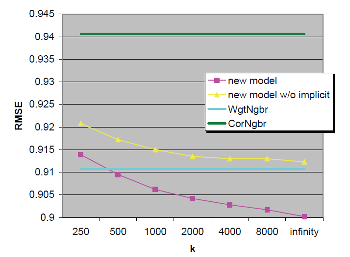
Figure 1: Comparison of neighborhood-based models. We measure the accuracy of the new model with and without implicit feedback. Accuracy is measured by RMSE on the Netflix test set, so lower values indicate better performance. RMSE is shown as a function of varying values of k k k, which dictates the neighborhood size. For reference, we present the accuracy of two prior models as two horizontal lines: the green line represents a popular method using Pearson correlations, and the cyan line represents a more recent neighborhood model.
图 1:基于邻域的模型比较。我们测量了新模型在有和没有隐式反馈情况下的准确性。准确性是通过 Netflix 测试集上的 RMSE 来衡量的,因此较低的值表示更好的性能。RMSE 显示为 k k k 的不同值的函数,这决定了邻域的大小。作为参考,我们展示了两个先前模型的准确性作为两条水平线:绿色线代表使用皮尔逊相关性的流行方法,青色线代表更近期的邻域模型。
Experimental results on the Netflix data with the new neighborhood model are presented in Fig. 1. We studied the model under different values of parameter k k k. The pink curve shows that accuracy monotonically improves with rising k k k values, as root mean squared error (RMSE) falls from 0.9139 for k = 250 k = 250 k=250 to 0.9002 for k = ∞ k = \infty k=∞ (Notice that since the Netflix data contains 17,770 movies, k = ∞ k = \infty k=∞ is equivalent to k = 17 , 770 k = 17,770 k=17,770, where all item-item relations are explored.) We repeated the experiments without using the implicit feedback, that is, dropping the c i j c_{ij} cij parameters from our model. The results depicted by the yellow curve show a significant decline in estimation accuracy, which widens as k k k grows. This demonstrates the value of incorporating implicit feedback into the model.
图 1 展示了新邻域模型在 Netflix 数据集上的实验结果。我们研究了不同 k k k 值对模型性能的影响:粉色曲线显示,随着 k k k 增大,模型精度单调提升,RMSE 从 k = 250 k = 250 k=250 时的 0.9139 降至 k = ∞ k = \infty k=∞ 时的 0.9002(注意:Netflix 数据集包含 17,770 部电影,因此 k = ∞ k = \infty k=∞ 等价于 k = 17 , 770 k = 17,770 k=17,770,即考虑所有物品间的关联)。我们还进行了"不使用隐式反馈"的对照实验(即从模型中移除 c i j c_{ij} cij 参数),黄色曲线显示,此时模型的估计精度显著下降,且随着 k k k 增大,精度差距进一步扩大------这证明了集成隐式反馈对模型的价值。
For comparison we provide the results of two previous neighborhood models. First is a correlation-based neighborhood model (following (3)), which is the most popular CF method in the literature. We denote this model as CorNgbr. Second is a newer model 2 that follows (4), which will be denoted as WgtNgbr. For both these two models, we tried to pick optimal parameters and neighborhood sizes, which were 20 for CorNgbr, and 50 for WgtNgbr. The results are depicted by the green and cyan lines. Notice that the k k k value (the x-axis) is irrelevant to these models, as their different notion of neighborhood makes neighborhood sizes incompatible. It is clear that the popular CorNgbr method is noticeably less accurate than the other neighborhood models, though its 0.9406 RMSE is still better than the published Netflix's Cinematch RMSE of 0.9514. On the opposite side, our new model delivers more accurate results even when compared with WgtNgbr, as long as the value of k k k is at least 500.
为进行对比,我们还展示了两种传统邻域模型的结果:第一种是基于相关系数的邻域模型(遵循公式 (3)),是文献中最常用的协同过滤方法,记为 CorNgbr;第二种是遵循公式 (4) 的较新模型2,记为 WgtNgbr。我们为这两种模型选择了最优参数和邻域大小:CorNgbr 的邻域大小为 20,WgtNgbr 的邻域大小为 50,结果分别用绿色和青色直线表示。需注意,x 轴的 k k k 值对这两种模型无意义(因其邻域定义与新模型不同,邻域大小无法直接比较)。显然,尽管 CorNgbr 的 RMSE(0.9406)仍优于 Netflix 公开的 Cinematch 系统(0.9514),但其精度显著低于其他邻域模型;而只要 k ≥ 500 k \geq 500 k≥500,我们提出的新模型即使与 WgtNgbr 相比,也能取得更高的精度。
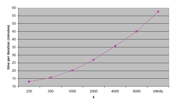
Figure 2: Running times (minutes) per iteration of the neighborhood model, as a function of the parameter k k k.
图 2:邻域模型每次迭代的运行时间(分钟),作为参数 k k k 的函数。
Finally, let us consider running time. Previous neighborhood models require very light pre-processing, though, WgtNgbr 2 requires solving a small system of equations for each provided prediction. The new model does involve pre-processing where parameters are estimated. However, online prediction is immediate by following rule (10). Pre-processing time grows with the value of k k k. Typical running times per iteration on the Netflix data, as measured on a single processor 3.4GHz Pentium 4 PC, are shown in Fig. 2.
最后,我们分析模型的运行时间:传统邻域模型的预处理计算量很小,但 WgtNgbr 2 在每次预测时都需要求解一个小型方程组;新模型的预处理阶段(参数估计)需要一定计算量,但在线预测时可直接通过公式 (10) 快速完成。预处理时间随 k k k 增大而增加,图 2 展示了"在 3.4GHz Pentium 4 单核处理器上"新模型在 Netflix 数据集中每次迭代的典型运行时间。
4. LATENT FACTOR MODELS REVISITED
4. 隐因子模型的再研究
As mentioned in Sec. 2.3, a popular approach to latent factor models is induced by an SVD-like lower rank decomposition of the ratings matrix. Each user u u u is associated with a user-factors vector p u ∈ R f p_u \in \mathbb{R}^f pu∈Rf, and each item i i i with an item-factors vector q i ∈ R f q_i \in \mathbb{R}^f qi∈Rf. Prediction is done by the rule:
如第 2.3 节所述,隐因子模型的一种常用方法是基于"评分矩阵的类 SVD 低秩分解":每个用户 u u u 对应一个用户因子向量 p u ∈ R f p_u \in \mathbb{R}^f pu∈Rf,每个物品 i i i 对应一个物品因子向量 q i ∈ R f q_i \in \mathbb{R}^f qi∈Rf,评分预测规则为:
r ^ u i = b u i + p u T q i ( 12 ) \hat{r}{ui} = b{ui} + p_u^T q_i \quad (12) r^ui=bui+puTqi(12)
Parameters are estimated by minimizing the associated squared error function (5). Funk 9 popularized gradient descent optimization, which was successfully practiced by many others 17, 18, 22. Henceforth, we will dub this basic model "SVD". We would like to extend the model by considering also implicit information. Following Paterek 17 and our work in the previous section, we suggest the following prediction rule:
r ^ u i = b u i + q i T ( ∣ R ( u ) ∣ − 1 2 ∑ j ∈ R ( u ) ( r u j − b u j ) x j + ∣ N ( u ) ∣ − 1 2 ∑ j ∈ N ( u ) y j ) ( 13 ) \begin{aligned} \hat{r}{ui} = b{ui} + q_i^T & \left( |R(u)|^{-\frac{1}{2}} \sum_{j \in R(u)} \left( r_{uj} - b_{uj} \right) x_j \right. \\ & \left. + |N(u)|^{-\frac{1}{2}} \sum_{j \in N(u)} y_j \right) \end{aligned} \quad (13) r^ui=bui+qiT ∣R(u)∣−21j∈R(u)∑(ruj−buj)xj+∣N(u)∣−21j∈N(u)∑yj (13)
Here, each item i i i is associated with three factor vectors q i q_i qi, x i x_i xi, y i ∈ R f y_i \in \mathbb{R}^f yi∈Rf. On the other hand, instead of providing an explicit parameterization for users, we represent users through the items that they prefer. Thus, the previous user factor p u p_u pu was replaced by the sum ∣ R ( u ) ∣ − 1 2 ∑ j ∈ R ( u ) ( r u j − b u j ) x j + ∣ N ( u ) ∣ − 1 2 ∑ j ∈ N ( u ) y j |R(u)|^{-\frac{1}{2}} \sum_{j \in R(u)} (r_{uj} - b_{uj}) x_j + |N(u)|^{-\frac{1}{2}} \sum_{j \in N(u)} y_j ∣R(u)∣−21∑j∈R(u)(ruj−buj)xj+∣N(u)∣−21∑j∈N(u)yj. This new model, which will be henceforth named "Asymmetric-SVD", offers several benefits:
其中,每个物品 i i i 对应三个因子向量 q i , x i , y i ∈ R f q_i, x_i, y_i \in \mathbb{R}^f qi,xi,yi∈Rf;与标准 SVD 模型不同,该模型不直接为用户设置参数,而是通过"用户偏好的物品"来表示用户------将标准 SVD 中的用户因子 p u p_u pu 替换为 ∣ R ( u ) ∣ − 1 2 ∑ j ∈ R ( u ) ( r u j − b u j ) x j + ∣ N ( u ) ∣ − 1 2 ∑ j ∈ N ( u ) y j |R(u)|^{-\frac{1}{2}} \sum_{j \in R(u)} (r_{uj} - b_{uj}) x_j + |N(u)|^{-\frac{1}{2}} \sum_{j \in N(u)} y_j ∣R(u)∣−21∑j∈R(u)(ruj−buj)xj+∣N(u)∣−21∑j∈N(u)yj。我们将这种新模型命名为"非对称 SVD(Asymmetric-SVD)",它具有以下优势:
Fewer parameters . Typically the number of users is much larger than the number of products. Thus, exchanging user-parameters with item-parameters lowers the complexity of the model. 参数数量更少:通常用户数量远大于物品数量,用物品参数替代用户参数可显著降低模型复杂度。
New users . Since Asymmetric-SVD does not parameterize users, we can handle new users as soon as they provide feedback to the system, without needing to re-train the model and estimate new parameters. Similarly, we can immediately exploit new ratings for updating user preferences. Notice that for new items we do have to learn new parameters. Interestingly, this asymmetry between users and items meshes well with common practices: systems need to provide immediate recommendations to new users who expect quality service. On the other hand, it is reasonable to require a waiting period before recommending items new to the system. As a side remark, it is worth mentioning that item-oriented neighborhood models exhibit the same desired asymmetry. 支持新用户:由于非对称 SVD 不为用户设置参数,新用户只要向系统提供反馈(显式评分或隐式偏好),即可直接获得推荐,无需重新训练模型或估计新参数;同理,用户的新评分也可立即用于更新其偏好表示。需注意,新物品仍需学习新参数------这种"用户与物品的非对称性"与实际应用场景高度契合:系统需要为新用户立即提供高质量推荐,而对新物品,用户通常可接受"等待一段时间再获取推荐"。值得一提的是,面向物品的邻域模型也具有这种理想的非对称性。
Explainability . Users expect a system to give a reason for its predictions, rather than facing "black box" recommendations. This not only enriches the user experience, but also encourages users to interact with the system, fix wrong impressions and improve long-term accuracy. In fact, the importance of explaining automated recommendations is widely recognized 11, 23. Latent factor models such as SVD face real difficulties to explain predictions. After all, a key to these models is abstracting users via an intermediate layer of user factors. This intermediate layer separates the computed predictions from past user actions and complicates explanations. However, the new Asymmetric-SVD model does not employ any level of abstraction on the users side. Hence, predictions are a direct function of past users' feedback. Such a framework allows identifying which of the past user actions are most influential on the computed prediction, thereby explaining predictions by most relevant actions. Once again, we would like to mention that item-oriented neighborhood models enjoy the same benefit. 可解释性:用户期望推荐系统能解释推荐理由,而非面对"黑箱"推荐。可解释性不仅能提升用户体验,还能鼓励用户与系统互动(如纠正错误认知),从而提高系统的长期精度。事实上,推荐系统的可解释性已被广泛认可为重要研究方向11, 23。传统 SVD 等隐因子模型的预测过程难以解释------其核心在于通过"用户因子"这一中间层对用户进行抽象,而该中间层将预测结果与用户过往行为隔离开来,导致解释困难。相比之下,非对称 SVD 模型对用户无任何抽象处理,预测结果是用户过往反馈的直接函数。这种框架可明确识别"对预测结果影响最大的用户过往行为",从而通过"最相关的行为"解释推荐理由。同样,面向物品的邻域模型也具有这一优势。
Efficient integration of implicit feedback . Prediction accuracy is improved by considering also implicit feedback, which provides an additional indication of user preferences. Obviously, implicit feedback becomes increasingly important for users that provide much more implicit feedback than explicit one. Accordingly, in rule (13) the implicit perspective becomes more dominant as ∣ N ( u ) ∣ |N(u)| ∣N(u)∣ increases and we have much implicit feedback. On the other hand, the explicit perspective becomes more significant when ∣ R ( u ) ∣ |R(u)| ∣R(u)∣ is growing and we have many explicit observations. Typically, a single explicit input would be more valuable than a single implicit input. The right conversion ratio, which represents how many implicit inputs are as significant as a single explicit input,is automatically learnt from the data by setting the relative values of the x j x_j xj and y j y_j yj parameters. 高效集成隐式反馈 :通过考虑隐式反馈(为用户偏好提供额外线索),模型预测精度得以提升。显然,对于"隐式反馈远多于显式反馈"的用户,隐式反馈的重要性会显著增加。在公式 (13) 中,随着 ∣ N ( u ) ∣ |N(u)| ∣N(u)∣ 增大(隐式反馈增多),隐式反馈对预测的影响会更显著;反之,当 ∣ R ( u ) ∣ |R(u)| ∣R(u)∣ 增大(显式评分增多),显式反馈的影响会更突出。通常,单个显式输入的价值高于单个隐式输入,而"多少个隐式输入等价于一个显式输入"的合理转换比例,会通过数据自动学习------具体表现为模型对 x j x_j xj 和 y j y_j yj 参数相对值的调整。
As usual, we learn the values of involved parameters by minimizing the regularized squared error function associated with (13):
与常规做法一致,我们通过最小化公式 (13) 对应的正则化平方误差函数来学习模型参数:
min q ∗ , x ∗ , y ∗ , b ∗ ∑ ( u , i ) ∈ K ( r u i − μ − b u − b i − q i T ( ∣ R ( u ) ∣ − 1 2 ∑ j ∈ R ( u ) ( r u j − b u j ) x j + ∣ N ( u ) ∣ − 1 2 ∑ j ∈ N ( u ) y j ) ) 2 + λ 5 ( b u 2 + b i 2 + ∥ q i ∥ 2 + ∑ j ∈ R ( u ) ∥ x j ∥ 2 + ∑ j ∈ N ( u ) ∥ y j ∥ 2 ) ( 14 ) \begin{aligned} & \min_{q_*, x_*, y_*, b_*} \sum_{(u, i) \in \mathcal{K}} \left( r_{ui} - \mu - b_u - b_i \right. \\ & \left. - q_i^T \left( |R(u)|^{-\frac{1}{2}} \sum_{j \in R(u)} \left( r_{uj} - b_{uj} \right) x_j + |N(u)|^{-\frac{1}{2}} \sum_{j \in N(u)} y_j \right) \right)^2 \\ & + \lambda_5 \left( b_u^2 + b_i^2 + \| q_i \|^2 + \sum_{j \in R(u)} \| x_j \|^2 + \sum_{j \in N(u)} \| y_j \|^2 \right) \end{aligned} \quad (14) q∗,x∗,y∗,b∗min(u,i)∈K∑(rui−μ−bu−bi−qiT ∣R(u)∣−21j∈R(u)∑(ruj−buj)xj+∣N(u)∣−21j∈N(u)∑yj 2+λ5 bu2+bi2+∥qi∥2+j∈R(u)∑∥xj∥2+j∈N(u)∑∥yj∥2 (14)
We employ a simple gradient descent scheme to solve the system. On the Netflix data we used 30 iterations, with step size of 0.002 and λ 5 = 0.04 \lambda_5 = 0.04 λ5=0.04.
Table 1: Comparison of SVD-based models: prediction accuracy is measured by RMSE on the Netflix test set for varying number of factors ( f f f). Asymmetric-SVD offers practical advantages over the known SVD model, while slightly improving accuracy. Best accuracy is achieved by SVD++, which directly incorporates implicit feedback into the SVD model.
表 1:基于 SVD 的模型对比。预测精度通过"Netflix 测试集上的 RMSE"衡量,结果随隐因子维度 f f f 变化。非对称 SVD 相比标准 SVD 具有实用优势,且精度略有提升;SVD++ 通过将隐式反馈直接集成到 SVD 模型中,取得了最高精度。
An important question is whether we need to give up some predictive accuracy in order to enjoy those aforementioned benefits of Asymmetric-SVD. We evaluated this on the Netflix data. As shown in Table 1, prediction quality of Asymmetric-SVD is actually slightly better than SVD. The improvement is likely thanks to accounting for implicit feedback. This means that one can enjoy the benefits that Asymmetric-SVD offers, without sacrificing prediction accuracy. As mentioned earlier, we do not really have much independent implicit feedback for the Netflix dataset. Thus, we expect that for real life systems with access to better types of implicit feedback (such as rental/purchase history), the new Asymmetric-SVD model would lead to even further improvements. Nevertheless, this still has to be demonstrated experimentally.
In fact, as far as integration of implicit feedback is concerned, we could get more accurate results by a more direct modification of (12), leading to the following model:
r ^ u i = b u i + q i T ( p u + ∣ N ( u ) ∣ − 1 2 ∑ j ∈ N ( u ) y j ) ( 15 ) \hat{r}{ui} = b{ui} + q_i^T \left( p_u + |N(u)|^{-\frac{1}{2}} \sum_{j \in N(u)} y_j \right) \quad (15) r^ui=bui+qiT pu+∣N(u)∣−21j∈N(u)∑yj (15)
Now, a user u u u is modeled as p u + ∣ N ( u ) ∣ − 1 2 ∑ j ∈ N ( u ) y j p_u + |N(u)|^{-\frac{1}{2}} \sum_{j \in N(u)} y_j pu+∣N(u)∣−21∑j∈N(u)yj. We use a free user-factors vector, p u p_u pu, much like in (12), which is learnt from the given explicit ratings. This vector is complemented by the sum ∣ N ( u ) ∣ − 1 2 ∑ j ∈ N ( u ) y j |N(u)|^{-\frac{1}{2}} \sum_{j \in N(u)} y_j ∣N(u)∣−21∑j∈N(u)yj, which represents the perspective of implicit feedback. We dub this model "SVD++". Similar models were discussed recently 3, 19. Model parameters are learnt by minimizing the associated squared error function through gradient descent. SVD++ does not offer the previously mentioned benefits of having less parameters, conveniently handling new users and readily explainable results. This is because we do abstract each user with a factors vector. However, as Table 1 indicates, SVD++ is clearly advantageous in terms of prediction accuracy. Actually, to our best knowledge, its results are more accurate than all previously published methods on the Netflix data. Nonetheless, in the next section we will describe an integrated model, which offers further accuracy gains.
在该模型中,用户 u u u 的表示为 p u + ∣ N ( u ) ∣ − 1 2 ∑ j ∈ N ( u ) y j p_u + |N(u)|^{-\frac{1}{2}} \sum_{j \in N(u)} y_j pu+∣N(u)∣−21∑j∈N(u)yj:其中 p u p_u pu 是与标准 SVD 模型(公式 (12))类似的"自由用户因子向量",通过显式评分学习得到;而 ∣ N ( u ) ∣ − 1 2 ∑ j ∈ N ( u ) y j |N(u)|^{-\frac{1}{2}} \sum_{j \in N(u)} y_j ∣N(u)∣−21∑j∈N(u)yj 则代表隐式反馈对用户偏好的补充。我们将该模型命名为"SVD++",近期已有相关类似模型的讨论3, 19。SVD++ 的参数通过梯度下降最小化对应的平方误差函数求解。需注意,SVD++ 不具备非对称 SVD 的优势(如参数更少、支持新用户、可解释性强)------因为它仍通过"用户因子向量"对用户进行抽象。但如表 1 所示,SVD++ 在预测精度上具有显著优势:据我们所知,其在 Netflix 数据集上的精度超过了所有已发表的方法。尽管如此,下一节我们将介绍一种"集成模型",可实现进一步的精度提升。
5. AN INTEGRATED MODEL
5. 集成模型
The new neighborhood model of Sec. 3 is based on a formal model, whose parameters are learnt by solving a least squares problem. An advantage of this approach is allowing easy integration with other methods that are based on similarly structured global cost functions. As explained in Sec. 1, latent factor models and neighborhood models nicely complement each other. Accordingly, in this section we will integrate the neighborhood model with our most accurate factor model -- SVD++. A combined model will sum the predictions of (10) and (15), thereby allowing neighborhood and factor models to enrich each other, as follows:
r ^ u i = μ + b u + b i + q i T ( p u + ∣ N ( u ) ∣ − 1 2 ∑ j ∈ N ( u ) y j ) + ∣ R k ( i ; u ) ∣ − 1 2 ∑ j ∈ R k ( i ; u ) ( r u j − b u j ) w i j + ∣ N k ( i ; u ) ∣ − 1 2 ∑ j ∈ N k ( i ; u ) c i j ( 16 ) \begin{array}{rl} \hat{r}{ui} &= \mu + b_u + b_i + q_i^T \left( p_u + |N(u)|^{-\frac{1}{2}} \sum{j \in N(u)} y_j \right) \\ & \quad + \left| R^k(i; u) \right|^{-\frac{1}{2}} \sum_{j \in R^k(i; u)} \left( r_{uj} - b_{uj} \right) w_{ij} + \left| N^k(i; u) \right|^{-\frac{1}{2}} \sum_{j \in N^k(i; u)} c_{ij} \end{array} \quad (16) r^ui=μ+bu+bi+qiT(pu+∣N(u)∣−21∑j∈N(u)yj)+ Rk(i;u) −21∑j∈Rk(i;u)(ruj−buj)wij+ Nk(i;u) −21∑j∈Nk(i;u)cij(16)
In a sense, rule (16) provides a 3-tier model for recommendations. The first tier, μ + b u + b i \mu + b_u + b_i μ+bu+bi, describes general properties of the item and the user, without accounting for any involved interactions. For example, this tier could argue that "The Sixth Sense" movie is known to be good, and that the rating scale of our user, Joe, tends to be just on average. The next tier, q i T ( p u + ∣ N ( u ) ∣ − 1 2 ∑ j ∈ N ( u ) y j ) q_i^T (p_u + |N(u)|^{-\frac{1}{2}} \sum_{j \in N(u)} y_j) qiT(pu+∣N(u)∣−21∑j∈N(u)yj), provides the interaction between the user profile and the item profile. In our example, it may find that "The Sixth Sense" and Joe are rated high on the Psychological Thrillers scale. The final "neighborhood tier" contributes fine grained adjustments that are hard to profile, such as the fact that Joe rated low the related movie "Signs".
从某种意义上说,公式 (16) 构成了一个"三层推荐模型":
第一层( μ + b u + b i \mu + b_u + b_i μ+bu+bi):描述物品和用户的全局属性,不考虑任何交互作用。例如,这一层可能反映"《第六感》(The Sixth Sense)是一部口碑良好的电影"以及"用户 Joe 的评分习惯接近平均水平"。
第二层( q i T ( p u + ∣ N ( u ) ∣ − 1 2 ∑ j ∈ N ( u ) y j ) q_i^T (p_u + |N(u)|^{-\frac{1}{2}} \sum_{j \in N(u)} y_j) qiT(pu+∣N(u)∣−21∑j∈N(u)yj)):捕捉用户画像与物品画像之间的交互作用。在上述例子中,这一层可能识别出"《第六感》和用户 Joe 在'心理惊悚片'维度上的匹配度很高"。
第三层(邻域层):提供"难以通过全局特征刻画的细粒度调整"。例如,若用户 Joe 对与《第六感》相关的电影《天兆》(Signs)评分较低,这一层会据此对 Joe 对《第六感》的预测评分进行微调。
Model parameters are determined by minimizing the associated regularized squared error function through gradient descent. Recall that e u i = def r u i − r ^ u i e_{ui} \stackrel{\text{def}}{=} r_{ui} - \hat{r}{ui} eui=defrui−r^ui. We loop over all known ratings in K K K. For a given training case r u i r{ui} rui, we modify the parameters by moving in the opposite direction of the gradient, yielding:
集成模型的参数通过"梯度下降最小化对应的正则化平方误差函数"求解。记预测误差 e u i = def r u i − r ^ u i e_{ui} \stackrel{\text{def}}{=} r_{ui} - \hat{r}_{ui} eui=defrui−r^ui,遍历所有已知评分 ( u , i ) ∈ K (u, i) \in K (u,i)∈K,沿梯度反方向更新参数,具体更新规则如下:
b u ← b u + γ 1 ⋅ ( e u i − λ 6 ⋅ b u ) b_u \leftarrow b_u + \gamma_1 \cdot \left( e_{ui} - \lambda_6 \cdot b_u \right) bu←bu+γ1⋅(eui−λ6⋅bu)
b i ← b i + γ 1 ⋅ ( e u i − λ 6 ⋅ b i ) b_i \leftarrow b_i + \gamma_1 \cdot \left( e_{ui} - \lambda_6 \cdot b_i \right) bi←bi+γ1⋅(eui−λ6⋅bi)
q i ← q i + γ 2 ⋅ ( e u i ⋅ ( p u + ∣ N ( u ) ∣ − 1 2 ∑ j ∈ N ( u ) y j ) − λ 7 ⋅ q i ) q_i \leftarrow q_i + \gamma_2 \cdot \left( e_{ui} \cdot \left( p_u + |N(u)|^{-\frac{1}{2}} \sum_{j \in N(u)} y_j \right) - \lambda_7 \cdot q_i \right) qi←qi+γ2⋅(eui⋅(pu+∣N(u)∣−21∑j∈N(u)yj)−λ7⋅qi)
p u ← p u + γ 2 ⋅ ( e u i ⋅ q i − λ 7 ⋅ p u ) p_u \leftarrow p_u + \gamma_2 \cdot \left( e_{ui} \cdot q_i - \lambda_7 \cdot p_u \right) pu←pu+γ2⋅(eui⋅qi−λ7⋅pu)
∀ j ∈ N ( u ) \forall j \in N(u) ∀j∈N(u):
y j ← y j + γ 2 ⋅ ( e u i ⋅ ∣ N ( u ) ∣ − 1 2 ⋅ q i − λ 7 ⋅ y j ) y_j \leftarrow y_j + \gamma_2 \cdot \left( e_{ui} \cdot |N(u)|^{-\frac{1}{2}} \cdot q_i - \lambda_7 \cdot y_j \right) yj←yj+γ2⋅(eui⋅∣N(u)∣−21⋅qi−λ7⋅yj)
∀ j ∈ R k ( i ; u ) \forall j \in R^k(i; u) ∀j∈Rk(i;u):
w i j ← w i j + γ 3 ⋅ ( ∣ R k ( i ; u ) ∣ − 1 2 ⋅ e u i ⋅ ( r u j − b u j ) − λ 8 ⋅ w i j ) w_{ij} \leftarrow w_{ij} + \gamma_3 \cdot \left( \left| R^k(i; u) \right|^{-\frac{1}{2}} \cdot e_{ui} \cdot \left( r_{uj} - b_{uj} \right) - \lambda_8 \cdot w_{ij} \right) wij←wij+γ3⋅( Rk(i;u) −21⋅eui⋅(ruj−buj)−λ8⋅wij)
∀ j ∈ N k ( i ; u ) \forall j \in N^k(i; u) ∀j∈Nk(i;u):
c i j ← c i j + γ 3 ⋅ ( ∣ N k ( i ; u ) ∣ − 1 2 ⋅ e u i − λ 8 ⋅ c i j ) c_{ij} \leftarrow c_{ij} + \gamma_3 \cdot \left( \left| N^k(i; u) \right|^{-\frac{1}{2}} \cdot e_{ui} - \lambda_8 \cdot c_{ij} \right) cij←cij+γ3⋅( Nk(i;u) −21⋅eui−λ8⋅cij)
50 factors
100 factors
200 factors
RMSE
0.8877
0.8870
0.8868
time/iteration
17min
20min
25min
Table 2: Performance of the integrated model. Prediction accuracy is improved by combining the complementing neighborhood and latent factor models. Increasing the number of factors contributes to accuracy, but also adds to running time.
When evaluating the method on the Netflix data, we used the following values for the meta parameters: γ 1 = γ 2 = 0.007 \gamma_1 = \gamma_2 = 0.007 γ1=γ2=0.007, γ 3 = 0.001 \gamma_3 = 0.001 γ3=0.001, λ 6 = 0.005 \lambda_6 = 0.005 λ6=0.005, λ 7 = λ 8 = 0.015 \lambda_7 = \lambda_8 = 0.015 λ7=λ8=0.015. It is beneficial to decrease step sizes (the γ \gamma γ's) by a factor of 0.9 after each iteration. The neighborhood size, k k k, was set to 300. Unlike the pure neighborhood model (10), here there is no benefit in increasing k k k, as adding neighbors covers more global information, which the latent factors already capture adequately. The iterative process runs for around 30 iterations till convergence. Table 2 summarizes the performance over the Netflix dataset for different number of factors. Once again, we report running times on a Pentium 4 PC for processing the 100 million ratings Netflix data. By coupling neighborhood and latent factor models together, and recovering signal from implicit feedback, accuracy of results is improved beyond other methods.
Recall that unlike SVD++, both the neighborhood model and Asymmetric-SVD allow a direct explanation of their recommendations, and do not require re-training the model for handling new users. Hence, when explainability is preferred over accuracy, one can follow very similar steps to integrate Asymmetric-SVD with the neighborhood model, thereby improving accuracy of the individual models while still maintaining the ability to reason about recommendations to end users.
So far, we have followed a common practice with the Netflix dataset to evaluate prediction accuracy by the RMSE measure. Achievable RMSE values on the Netflix test data lie in a quite narrow range. A simple prediction rule, which estimates r u i r_{ui} rui as the mean rating of movie i i i, will result in R M S E = 1.053 RMSE = 1.053 RMSE=1.053. Notice that this rule represents a sensible "best sellers list" approach, where the same recommendation applies to all users. By applying personalization, more accurate predictions are obtained. This way, Netflix Cinematch system could achieve a RMSE of 0.9514. In this paper, we suggested methods that lower the RMSE to 0.8870. In fact, by blending several solutions, we could reach a RMSE of 0.8645. Nonetheless, none of the 3,400 teams actively involved in the Netflix Prize competition could reach, as of 20 months into the competition, lower RMSE levels, despite the big incentive of winning a 1 M 1M 1M Grand Prize. Thus, the range of attainable RMSEs is seemingly compressed, with less than 20% gap between a naive nonpersonalized approach and the best known CF results. Successful improvements of recommendation quality depend on achieving the elusive goal of enhancing users' satisfaction. Thus, a crucial question is: what effect on user experience should we expect by lowering the RMSE by, say, 10%? For example, is it possible that a solution with a slightly better RMSE will lead to completely different and better recommendations? This is central to justifying research on accuracy improvements in recommender systems. We would like to shed some light on the issue, by examining the effect of lowered RMSE on a practical situation.
截至目前,我们遵循 Netflix 数据集的常规评估方式,使用 RMSE 衡量预测精度。但 Netflix 测试集上"可实现的 RMSE 范围非常狭窄":例如,"将 r u i r_{ui} rui 预测为电影 i i i 的平均评分"这一简单规则(对应"畅销榜单"式的非个性化推荐)的 RMSE 为 1.053;通过个性化技术,Netflix 的 Cinematch 系统将 RMSE 降至 0.9514;本文提出的方法进一步将 RMSE 降至 0.8870,若融合多种方案甚至可达到 0.8645。然而,尽管有 100 万美元大奖的激励,在 Netflix Prize 竞赛开展 20 个月后,3400 支参赛队伍中仍无任何一支能将 RMSE 进一步降低。由此可见,"可实现的 RMSE 范围"具有明显的压缩性------从"朴素非个性化方法"到"已知最优协同过滤方法"的 RMSE 差距不足 20%。推荐系统的核心目标是提升用户满意度,因此一个关键问题应运而生:例如,将 RMSE 降低 10%,会对用户体验产生何种影响?精度略高的模型是否可能生成"完全不同且质量更优"的推荐?这一问题是"研究推荐系统精度提升"的核心合理性依据。为解答该问题,我们将通过"实际场景测试",分析 RMSE 降低对推荐效果的影响。
A common case facing recommender systems is providing "top K recommendations". That is, the system needs to suggest the top K products to a user. For example, recommending the user a few specific movies which are supposed to be most appealing to him. We would like to investigate the effect of lowering the RMSE on the quality of top K recommendations. Somewhat surprisingly, the Netflix dataset can be used to evaluate this.
推荐系统的一个常见应用场景是"Top-K 推荐"------即向用户推荐"预测最符合其偏好的 K 个产品"(例如,向用户推荐几部最可能吸引他的电影)。我们希望通过该场景,研究"RMSE 降低"对 Top-K 推荐质量的影响。令人意外的是,Netflix 数据集可用于开展这类评估。
Recall that in addition to the test set, Netflix also provided a validation set for which the true ratings are published. We used all 5-star ratings from the validation set as a proxy for movies that interest users. Our goal is to find the relative place of these "interesting movies" within the total order of movies sorted by predicted ratings for a specific user. To this end, for each such movie i i i, rated 5-stars by user u u u, we select 1000 additional random movies and predict the ratings by u u u for i i i and for the other 1000 movies. Finally, we order the 1001 movies based on their predicted rating, in a decreasing order. This simulates a situation where the system needs to recommend movies out of 1001 available ones. Thus, those movies with the highest predictions will be recommended to user u u u. Notice that the 1000 movies are random, some of which may be of interest to user u u u, but most of them are probably of no interest to u u u. Hence, the best hoped result is that i i i (for which we know u u u gave the highest rating of 5) will precede the rest 1000 random movies, thereby improving the appeal of a top-K recommender. There are 1001 different possible ranks for i i i, ranging from the best case where none (0%) of the random movies appears before i i i, to the worst case where all (100%) of the random movies appear before i i i in the sorted order. Overall, the validation set contains 384,573 5-star ratings. For each of them (separately) we draw 1000 random movies, predict associated ratings, and derive a ranking between 0% to 100%. Then, the distribution of the 384,573 ranks is analyzed. (Remark: since the number 1000 is arbitrary, reported results are in percentiles (0%--100%), rather than in absolute ranks (0--1000).)
显然,1000 部随机电影中可能包含少量用户感兴趣的影片,但大多数与用户偏好无关。因此,理想结果是"电影 i i i(已知用户给 5 星)排在 1000 部随机电影之前"------这能直接提升 Top-K 推荐的吸引力。电影 i i i 共有 1001 种可能的排名(按百分比计):最佳情况是 0%(无随机电影排在 i i i 之前),最差情况是 100%(所有随机电影都排在 i i i 之前)。验证集中共有 384,573 条 5 星评分记录,我们对每条记录均执行上述步骤,得到 384,573 个"0%--100%"的排名结果,最终分析这些排名的分布情况(注:由于 1000 是任意选择的数量,结果以百分位(0%--100%)呈现,而非绝对排名(0--1000))。
We used this methodology to evaluate five different methods. The first method is the aforementioned non-personalized prediction rule, which employs movie means to yield R M S E = 1.053 RMSE = 1.053 RMSE=1.053. Henceforth, it will be denoted as MovieAvg. The second method is a correlation-based neighborhood model, which is the most popular approach in the CF literature. As mentioned in Sec. 3, it achieves a RMSE of 0.9406 on the test set, and was named CorNgbr. The third method is the improved neighborhood approach of 2, which we named WgtNgbr and could achieve R M S E = 0.9107 RMSE = 0.9107 RMSE=0.9107 on the test set. Fourth is the SVD latent factor model, with 100 factors thereby achieving R M S E = 0.9025 RMSE = 0.9025 RMSE=0.9025 as reported in Table 1. Finally, we consider our most accurate method, the integrated model, with 100 factors, achieving R M S E = 0.8870 RMSE = 0.8870 RMSE=0.8870 as shown in Table 2.
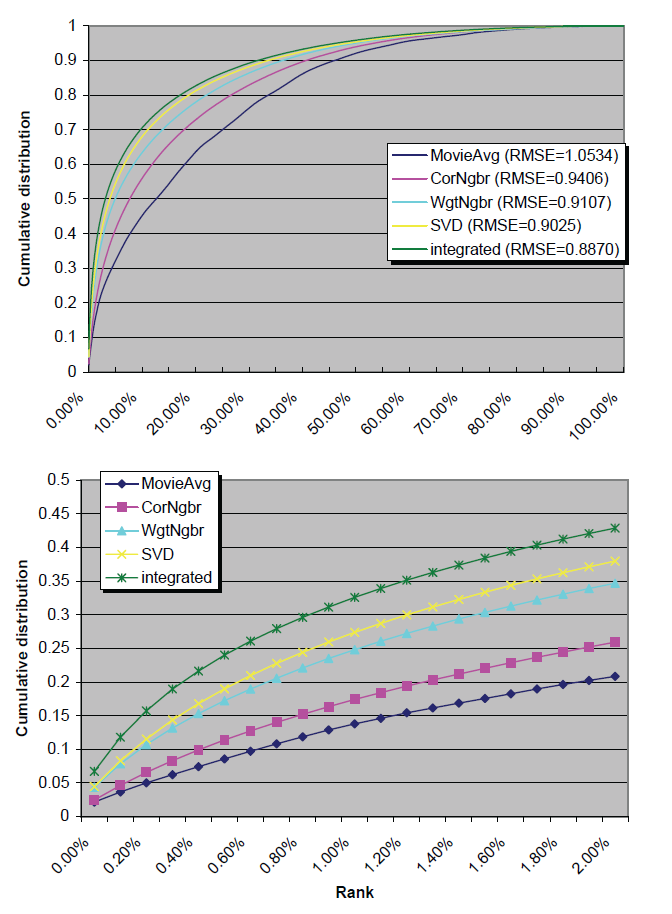
Figure 3: Comparing the performance of five methods on a top-K recommendation task, where a few products need to be suggested to a user. Values on the x x x-axis stand for the percentile ranking of a 5-star rated movie; lower values represent more successful recommendations. We experiment with 384,573 cases and show the cumulative distribution of the results. The lower plot concentrates on the more relevant region, pertaining to low x x x-axis values. The plot shows that the integrated method has the highest probability of obtaining low values on the x x x-axis. On the other hand, the non-personalized MovieAvg method and the popular correlation-based neighborhood method (CorNbr) achieve the lowest probabilities.
图 3:比较五种方法在 top-K 推荐任务中的性能,其中需要向用户推荐一些产品。x 轴上的值代表 5 星级电影的百分位排名;较低的值代表更成功的推荐。我们进行了 384,573 个案例的实验,并展示了结果的累积分布。下图集中在更相关的区域,涉及 x x x 轴上的低值。图表显示,集成方法在 x x x 轴上获得低值的概率最高。另一方面,非个性化的 MovieAvg 方法和流行的基于相关性的邻域方法(CorNbr)获得最低概率。
Figure 3(top) plots the cumulative distribution of the computed percentile ranks for the five methods over the 384,573 evaluated cases. Clearly, all methods would outperform a random/constant prediction rule, which would have resulted in a straight line connecting the bottom-left and top-right corners. Also, the figure exhibits an ordering of the methods by their strength. In order to achieve a better understanding, let us zoom in on the head of the x-axis, which represents top-K recommendations. After all, in order to get into the top-K recommendations, a product should be ranked before almost all others. For example, if 600 products are considered, and three of them will be suggested to the user, only those ranked 0.5% or lower are relevant. In a sense, there is no difference between placing a desired 5-star movie at the top 5%, top 20% or top 80%, as none of them is good enough to be presented to the user. Accordingly, Fig. 3(bottom), plots the cumulative ranks distribution between 0% and 2% (top 20 ranked items out of 1000).
As the figure shows, there are very significant differences among the methods. For example, the integrated method has a probability of 0.067 to place a 5-star movie before all other 1000 movies (rank = 0%). This is more than three times better than the chance of the MovieAvg method to achieve the same. In addition, it is 2.8 times better than the chance of the popular CorNgbr to achieve the same. The other two methods, WgtNgbr and SVD, have a probability of around 0.043 to achieve the same. The practical interpretation is that if about 0.1% of the items are selected to be suggested to the user, the integrated method has a significantly higher chance to pick a specified 5-star rated movie. Similarly, the integrated method has a probability of 0.157 to place the 5-star movie before at least 99.8% of the random movies (rank ≤ 0.2%). For comparison, MovieAvg and CorNgbr have much slimmer chances of achieving the same: 0.050 and 0.065, respectively. The remaining two methods, WgtNgbr and SVD, lie between with probabilities of 0.107 and 0.115, respectively. Thus, if one movie out of 500 is to be suggested, its probability of being a specific 5-stars rated one becomes noticeably higher with the integrated model.
We are encouraged, even somewhat surprised, by the results. It is evident that small improvements in RMSE translate into significant improvements in quality of the top K products. In fact, based on RMSE differences, we did not expect the integrated model to deliver such an emphasized improvement in the test. Similarly, we did not expect the very weak performance of the popular correlation based neighborhood scheme, which could not improve much upon a non-personalized scheme.
This work proposed improvements to two of the most popular approaches to Collaborative Filtering. First, we suggested a new neighborhood based model, which unlike previous neighborhood methods, is based on formally optimizing a global cost function. This leads to improved prediction accuracy, while maintaining merits of the neighborhood approach such as explainability of predictions and ability to handle new users without re-training the model. Second, we introduced extensions to SVD-based latent factor models that allow improved accuracy by integrating implicit feedback into the model. One of the models also provides advantages that are usually regarded as belonging to neighborhood models, namely, an ability to explain recommendations and to handle new users seamlessly. In addition, the new neighborhood model enables us to derive, for the first time, an integrated model that combines the neighborhood and the latent factor models. This is helpful for improving system performance, as the neighborhood and latent factor models address the data at different levels and complement each other.
Quality of a recommender system is expressed through multiple dimensions including: accuracy, diversity, ability to surprise with unexpected recommendations, explainability, appropriate top-K recommendations, and computational efficiency. Some of those criteria are relatively easy to measure, such as accuracy and efficiency that were addressed in this work. Some other aspects are more elusive and harder to quantify. We suggested a novel approach for measuring the success of a top-K recommender, which is central to most systems where a few products should be suggested to each user. It is notable that evaluating top-K recommenders significantly sharpens the differences between the methods, beyond what a traditional accuracy measure could show.
A major insight beyond this work is that improved recommendation quality depends on successfully addressing different aspects of the data. A prime example is using implicit user feedback to extend models' quality, which our methods facilitate. Evaluation of this was based on a very limited form of implicit feedback, which was available within the Netflix dataset. This was enough to show a marked improvement, but further experimentation is needed with better sources of implicit feedback, such as purchase/rental history. Other aspects of the data that may be integrated to improve prediction quality are content information like attributes of users or products, or dates associated with the ratings, which may help to explain shifts in user preferences.
The author thanks Suhrid Balakrishnan, Robert Bell and Stephen North for their most helpful remarks.
作者感谢 Suhrid Balakrishnan、Robert Bell 和 Stephen North 提供的有益建议。
8. REFERENCES
8. 参考文献
1 G. Adomavicius and A. Tuzhilin, "Towards the Next Generation of Recommender Systems: A Survey of the State-of-the-Art and Possible Extensions", IEEE Transactions on Knowledge and Data Engineering 17 (2005), 634--749.
2 R. Bell and Y. Koren, "Scalable Collaborative Filtering with Jointly Derived Neighborhood Interpolation Weights", IEEE International Conference on Data Mining (ICDM'07), pp. 43--52, 2007.
3 R. Bell and Y. Koren, "Lessons from the Netflix Prize Challenge", SIGKDD Explorations 9 (2007), 75--79.
4 R. M. Bell, Y. Koren and C. Volinsky, "Modeling Relationships at Multiple Scales to Improve Accuracy of Large Recommender Systems", Proc. 13th ACM SIGKDD International Conference on Knowledge Discovery and Data Mining, 2007.
5 J. Bennet and S. Lanning, "The Netflix Prize", KDD Cup and Workshop, 2007. www.netflixprize.com.
6 J. Canny, "Collaborative Filtering with Privacy via Factor Analysis", Proc. 25th ACM SIGIR Conf. on Research and Development in Information Retrieval (SIGIR'02), pp. 238--245, 2002.
7 D. Blei, A. Ng, and M. Jordan, "Latent Dirichlet Allocation", Journal of Machine Learning Research 3 (2003), 993--1022.
8 S. Deerwester, S. Dumais, G. W. Furnas, T. K. Landauer and R. Harshman, "Indexing by Latent Semantic Analysis", Journal of the Society for Information Science 41 (1990), 391--407.
10 D. Goldberg, D. Nichols, B. M. Oki and D. Terry, "Using Collaborative Filtering to Weave an Information Tapestry", Communications of the ACM 35 (1992), 61--70.
11 J. L. Herlocker, J. A. Konstan and J. Riedl, "Explaining Collaborative Filtering Recommendations", Proc. ACM conference on Computer Supported Cooperative Work, pp. 241--250, 2000.
12 J. L. Herlocker, J. A. Konstan, A. Borchers and John Riedl, "An Algorithmic Framework for Performing Collaborative Filtering", Proc. 22nd ACM SIGIR Conference on Information Retrieval, pp. 230--237, 1999.
13 T. Hofmann, "Latent Semantic Models for Collaborative Filtering", ACM Transactions on Information Systems 22 (2004), 89--115.
14 D. Kim and B. Yum, "Collaborative Filtering Based on Iterative Principal Component Analysis", Expert Systems with Applications 28 (2005), 823--830.
15 G. Linden, B. Smith and J. York, "Amazon.com Recommendations: Item-to-item Collaborative Filtering", IEEE Internet Computing 7 (2003), 76--80.
16 D.W. Oard and J. Kim, "Implicit Feedback for Recommender Systems", Proc. 5th DELOS Workshop on Filtering and Collaborative Filtering, pp. 31--36, 1998.
17 A. Paterek, "Improving Regularized Singular Value Decomposition for Collaborative Filtering", Proc. KDD Cup and Workshop, 2007.
18 R. Salakhutdinov, A. Mnih and G. Hinton, "Restricted Boltzmann Machines for Collaborative Filtering", Proc. 24th Annual International Conference on Machine Learning, pp. 791--798, 2007.
19 R. Salakhutdinov and A. Mnih, "Probabilistic Matrix Factorization", Advances in Neural Information Processing Systems 20 (NIPS'07), pp. 1257--1264, 2008.
20 B. M. Sarwar, G. Karypis, J. A. Konstan, and J. Riedl, "Application of Dimensionality Reduction in Recommender System -- A Case Study", WEBKDD'2000.
21 B. Sarwar, G. Karypis, J. Konstan and J. Riedl, "Item-based Collaborative Filtering Recommendation Algorithms", Proc. 10th International Conference on the World Wide Web, pp. 285-295, 2001.
22 G. Takacs, I. Pilaszy, B. Nemeth and D. Tikk, "Major Components of the Gravity Recommendation System", SIGKDD Explorations 9 (2007), 80--84.
23 N. Tintarev and J. Masthoff, "A Survey of Explanations in Recommender Systems", ICDE'07 Workshop on Recommender Systems and Intelligent User Interfaces, 2007.
via:
Factorization meets the neighborhood | Proceedings of the 14th ACM SIGKDD international conference on Knowledge discovery and data mining https://dl.acm.org/doi/10.1145/1401890.1401944