python
from collections import defaultdict
import multiprocessing
import matplotlib.pyplot as plt
import torch
from tensordict.nn import TensorDictModule
from tensordict.nn.distributions import NormalParamExtractor
from torch import nn
from torchrl.collectors import SyncDataCollector
from torchrl.data.replay_buffers import ReplayBuffer
from torchrl.data.replay_buffers.samplers import SamplerWithoutReplacement
from torchrl.data.replay_buffers.storages import LazyTensorStorage
from torchrl.envs import (Compose, DoubleToFloat, ObservationNorm, StepCounter, TransformedEnv)
from torchrl.envs.libs.gym import GymEnv
from torchrl.envs.utils import check_env_specs, ExplorationType, set_exploration_type
from torchrl.modules import ProbabilisticActor, TanhNormal, ValueOperator
from torchrl.objectives import ClipPPOLoss
from torchrl.objectives.value import GAE
from tqdm import tqdm
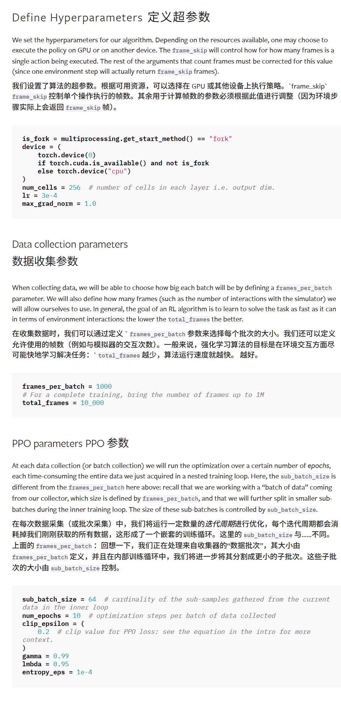
# 定义超参数
'''
我们设置了算法的超参数。根据可用资源,可以选择在 GPU 或其他设备上执行策略。`frame_skip` frame_skip 控制单个操作执行的帧数。其余用于计算帧数的参数必须根据此值进行调整(因为环境步骤实际上会返回 frame_skip 帧)。
'''
is_fork = multiprocessing.get_start_method() == "fork"
device = (
torch.device(0)
if torch.cuda.is_available() and not is_fork
else torch.device("cpu")
)
num_cells = 256
lr = 3e-4
max_grad_norm = 1.0
# collector参数
'''
在收集数据时,我们可以通过定义 ` frames_per_batch 参数来选择每个批次的大小。我们还可以定义允许使用的帧数(例如与模拟器的交互次数)。一般来说,强化学习算法的目标是在环境交互方面尽可能快地学习解决任务:` total_frames 越少,算法运行速度就越快。 越好。
'''
frames_per_batch = 1000
total_frames = 10000
# PPO参数
'''
At each data collection (or batch collection) we will run the optimization over a certain number of epochs, each time-consuming the entire data we just acquired in a nested training loop. Here, the sub_batch_size is different from the frames_per_batch here above: recall that we are working with a "batch of data" coming from our collector, which size is defined by frames_per_batch, and that we will further split in smaller sub-batches during the inner training loop. The size of these sub-batches is controlled by sub_batch_size.
'''
sub_batch_size = 64
num_epochs = 10
clip_epsilon = 0.2
gamma = 0.99
lmbda = 0.95
entropy_eps = 1e-4
# 环境
base_env = GymEnv("InvertedPendulum-v4", device=device)
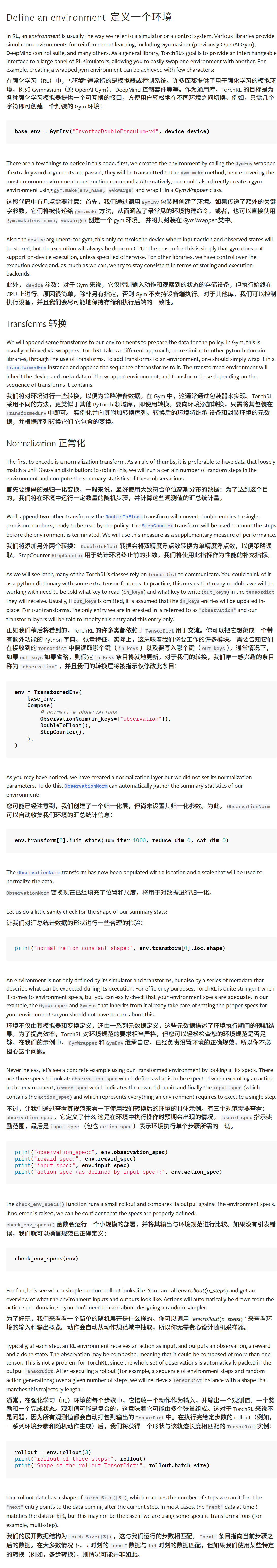
env = TransformedEnv(base_env, Compose(ObservationNorm(in_keys=["observation"]), DoubleToFloat(), StepCounter()))
env.transform[0].init_stats(num_iter=1000, reduce_dim=0, cat_dim=0)
print("normalization constant shape:", env.transform[0].loc.shape)
print("observation_spec:", env.observation_spec)
print("reward_spec:", env.reward_spec)
print("input_spec:", env.input_spec)
print("action_spec (as defined by input_spec):", env.action_spec)
check_env_specs(env)
rollout = env.rollout(3)
print("rollout of three steps:", rollout)
print("Shape of the rollout TensorDict:", rollout.batch_size)
# 策略
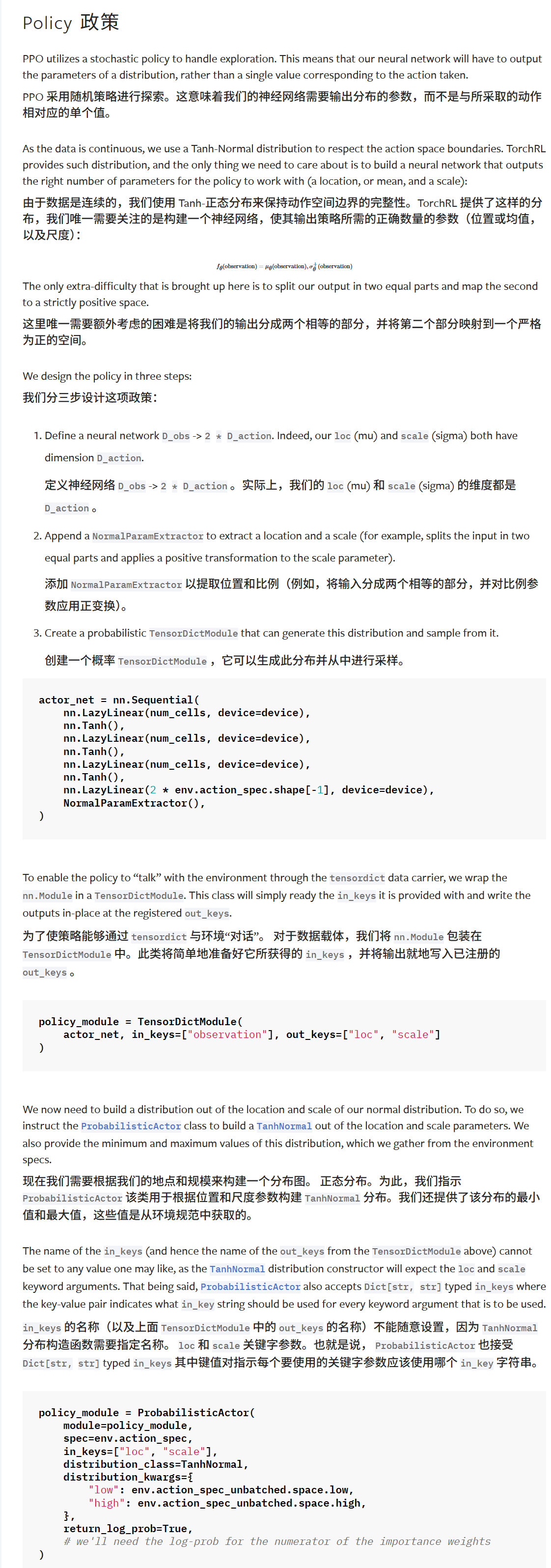
actor_net = nn.Sequential(
nn.LazyLinear(num_cells, device =device),
nn.Tanh(),
nn.LazyLinear(num_cells, device =device),
nn.Tanh(),
nn.LazyLinear(num_cells, device =device),
nn.Tanh(),
nn.LazyLinear(2 * env.action_spec.shape[-1], device =device),
NormalParamExtractor(),
)
policy_module = TensorDictModule(actor_net, in_keys=["observation"], out_keys=["loc", "scale"])
policy_module = ProbabilisticActor(
module = policy_module,
spec = env.action_spec,
in_keys=["loc", "scale"],
distribution_class = TanhNormal,
distribution_kwargs = {
"low": env.action_spec_unbatched.space.low,
"high": env.action_spec_unbatched.space.high,
},
return_log_prob = True,
)
# 价值
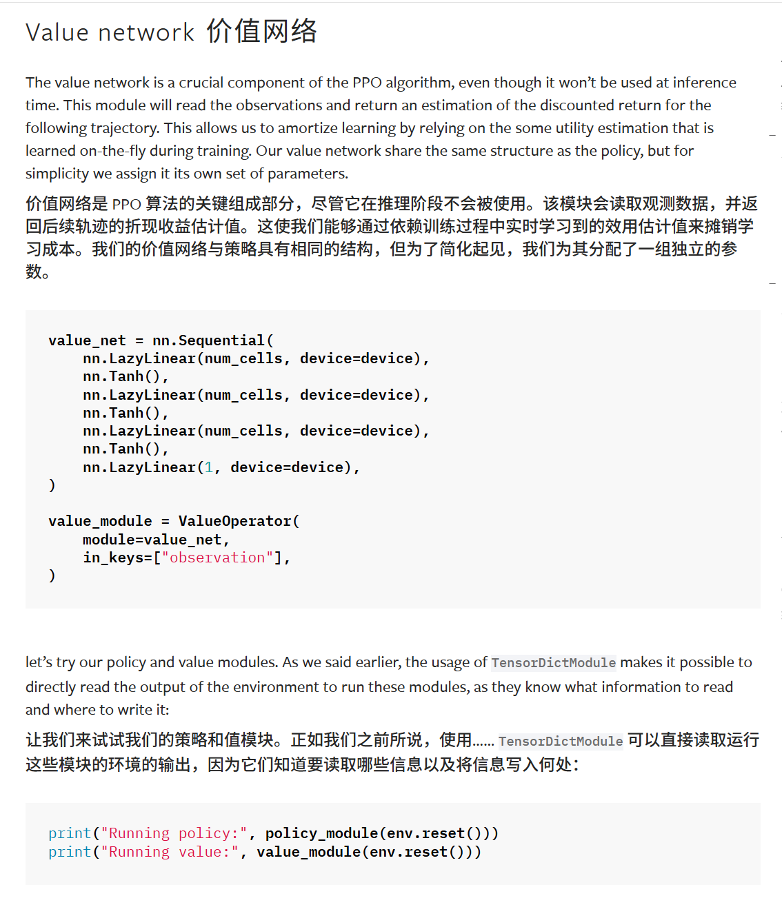
value_net = nn.Sequential(
nn.LazyLinear(num_cells, device =device),
nn.Tanh(),
nn.LazyLinear(num_cells, device =device),
nn.Tanh(),
nn.LazyLinear(num_cells, device =device),
nn.Tanh(),
nn.LazyLinear(1, device =device),
)
value_module = ValueOperator(
module=value_net,
in_keys=["observation"],
)
print("Running policy:", policy_module(env.reset()))
print("Running value:", value_module(env.reset()))
# 数据收集器
collector = SyncDataCollector(
env,
policy_module,
total_frames=total_frames,
frames_per_batch=frames_per_batch,
device=device,
)
# 缓冲区
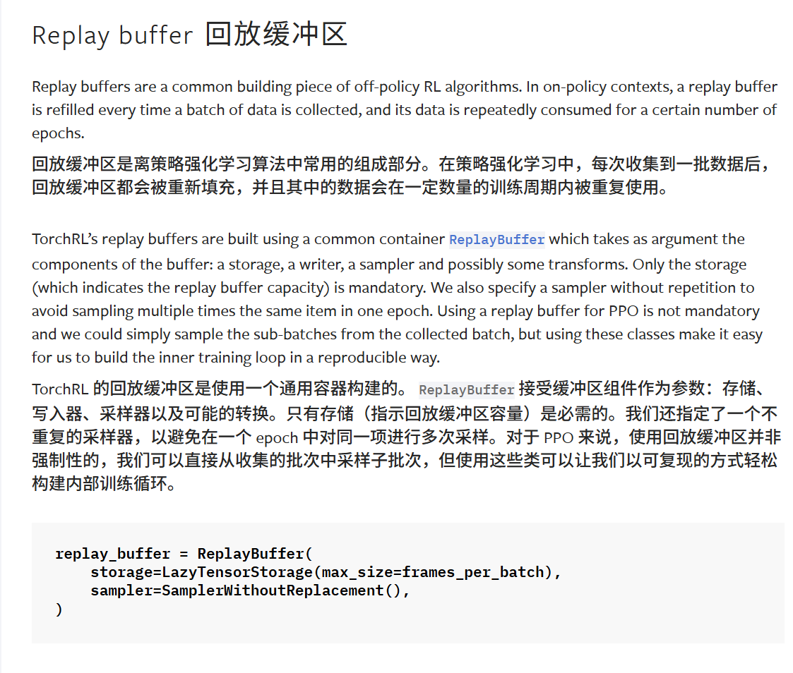
replay_buffer = ReplayBuffer(
storage=LazyTensorStorage(max_size=frames_per_batch),
sampler=SamplerWithoutReplacement(),
)
# 损失函数
advantage_module = GAE(gamma=gamma, lmbda=lmbda, value_network=value_module,average_gae=True)
loss_module = ClipPPOLoss(
actor_network=policy_module,
critic_network=value_module,
clip_epsilon=clip_epsilon,
entropy_bonus=entropy_eps,
critic_coeff=1.0,
loss_critic_type="smooth_l1",
)
optim = torch.optim.Adam(loss_module.parameters(), lr=lr)
scheduler = torch.optim.lr_scheduler.CosineAnnealingLR(optim,
total_frames //frames_per_batch, 0.0)
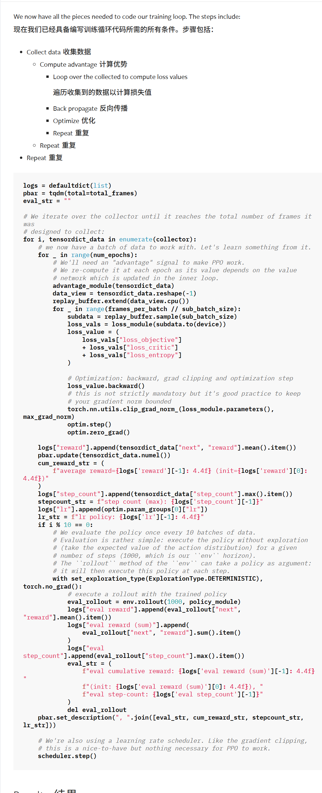
# 训练循环
logs = defaultdict(list)
pbar = tqdm(total=total_frames)
eval_str = ""
# We iterate over the collector until it reaches the total number of frames it was
# designed to collect:
for i, tensordict_data in enumerate(collector):
# we now have a batch of data to work with. Let's learn something from it.
for _ in range(num_epochs):
# We'll need an "advantage" signal to make PPO work.
# We re-compute it at each epoch as its value depends on the value
# network which is updated in the inner loop.
advantage_module(tensordict_data)
data_view = tensordict_data.reshape(-1)
replay_buffer.extend(data_view.cpu())
for _ in range(frames_per_batch // sub_batch_size):
subdata = replay_buffer.sample(sub_batch_size)
loss_vals = loss_module(subdata.to(device))
loss_value = (
loss_vals["loss_objective"]
+ loss_vals["loss_critic"]
+ loss_vals["loss_entropy"]
)
# Optimization: backward, grad clipping and optimization step
loss_value.backward()
# this is not strictly mandatory but it's good practice to keep
# your gradient norm bounded
torch.nn.utils.clip_grad_norm_(loss_module.parameters(), max_grad_norm)
optim.step()
optim.zero_grad()
logs["reward"].append(tensordict_data["next", "reward"].mean().item())
pbar.update(tensordict_data.numel())
cum_reward_str = (
f"average reward={logs['reward'][-1]: 4.4f} (init={logs['reward'][0]: 4.4f})"
)
logs["step_count"].append(tensordict_data["step_count"].max().item())
stepcount_str = f"step count (max): {logs['step_count'][-1]}"
logs["lr"].append(optim.param_groups[0]["lr"])
lr_str = f"lr policy: {logs['lr'][-1]: 4.4f}"
if i % 10 == 0:
# We evaluate the policy once every 10 batches of data.
# Evaluation is rather simple: execute the policy without exploration
# (take the expected value of the action distribution) for a given
# number of steps (1000, which is our ``env`` horizon).
# The ``rollout`` method of the ``env`` can take a policy as argument:
# it will then execute this policy at each step.
with set_exploration_type(ExplorationType.DETERMINISTIC), torch.no_grad():
# execute a rollout with the trained policy
eval_rollout = env.rollout(1000, policy_module)
logs["eval reward"].append(eval_rollout["next", "reward"].mean().item())
logs["eval reward (sum)"].append(
eval_rollout["next", "reward"].sum().item()
)
logs["eval step_count"].append(eval_rollout["step_count"].max().item())
eval_str = (
f"eval cumulative reward: {logs['eval reward (sum)'][-1]: 4.4f} "
f"(init: {logs['eval reward (sum)'][0]: 4.4f}), "
f"eval step-count: {logs['eval step_count'][-1]}"
)
del eval_rollout
pbar.set_description(", ".join([eval_str, cum_reward_str, stepcount_str, lr_str]))
# We're also using a learning rate scheduler. Like the gradient clipping,
# this is a nice-to-have but nothing necessary for PPO to work.
scheduler.step()
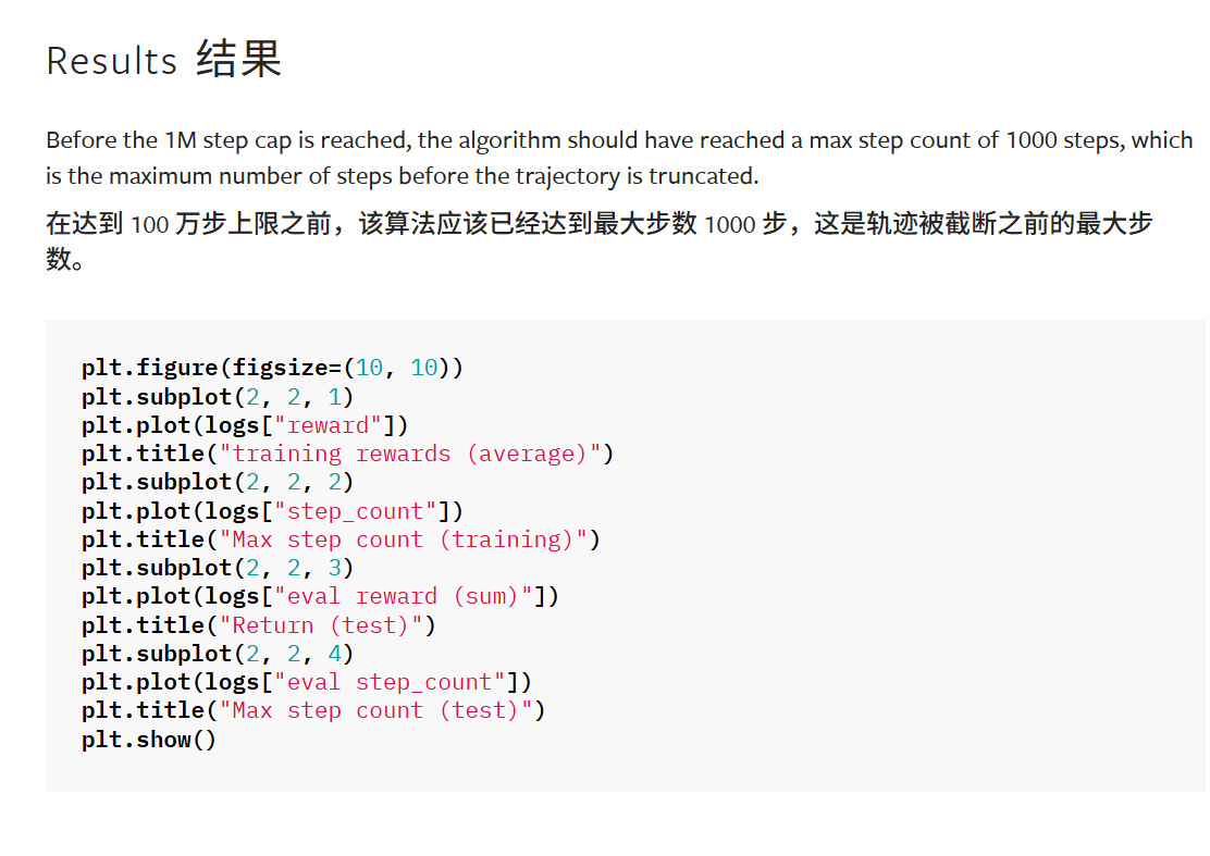
# 结果plt.figure(figsize=(10, 10))
plt.subplot(2, 2, 1)
plt.plot(logs["reward"])
plt.title("training rewards (average)")
plt.subplot(2, 2, 2)
plt.plot(logs["step_count"])
plt.title("Max step count (training)")
plt.subplot(2, 2, 3)
plt.plot(logs["eval reward (sum)"])
plt.title("Return (test)")
plt.subplot(2, 2, 4)
plt.plot(logs["eval step_count"])
plt.title("Max step count (test)")
plt.show()TorchRL 强化学习(PPO)教程
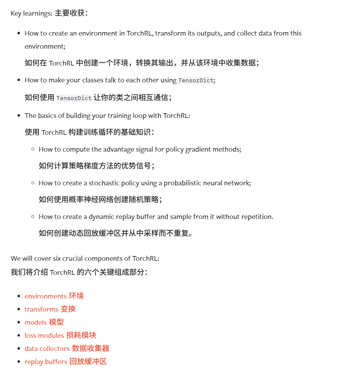
整体思路上还是和上一节的类似;
包括:环境(变换),模型,损失函数,数据收集器,回放缓冲区,日志,训练loop
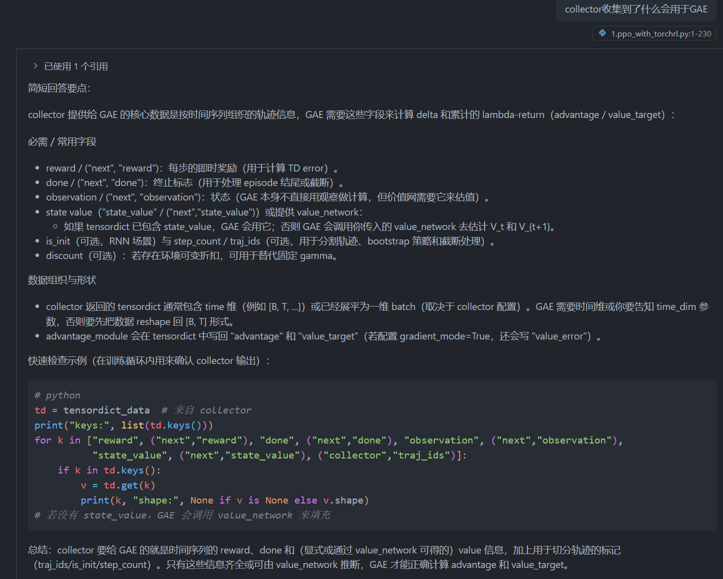
用的算法是PPO之前也已经提到过,涉及到了GAE,也就是
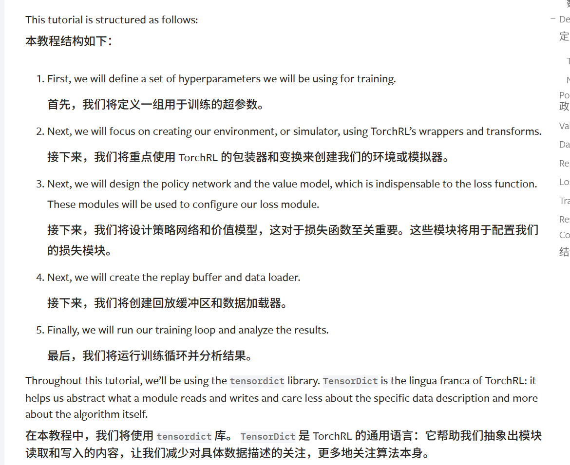
1.导包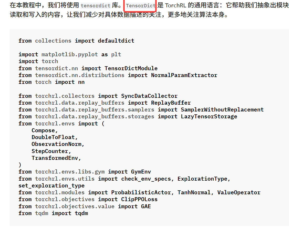
2.超参数
3.环境(包括TransformedEnv
4.策略 (包括NN架构,输出输出,概率分布
5.价值 (包括NN架构,输入
6.数据收集器 (和之前类似

7.Replaybuffer (策略可以由不重复采样
8.损失函数 (这里用的是PPO-Clip
涉及到了GAE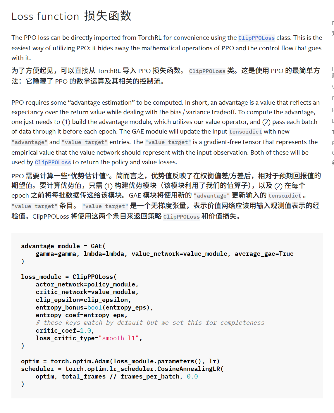
9.训练循环
已经给出了伪代码,需要注意的是这里的每一层for循环代表什么
10.打印结果
总结:
问题
为什么会用到大量CPU,其实可以看到这里的环境或者simulator是在CPU上面运行,即使
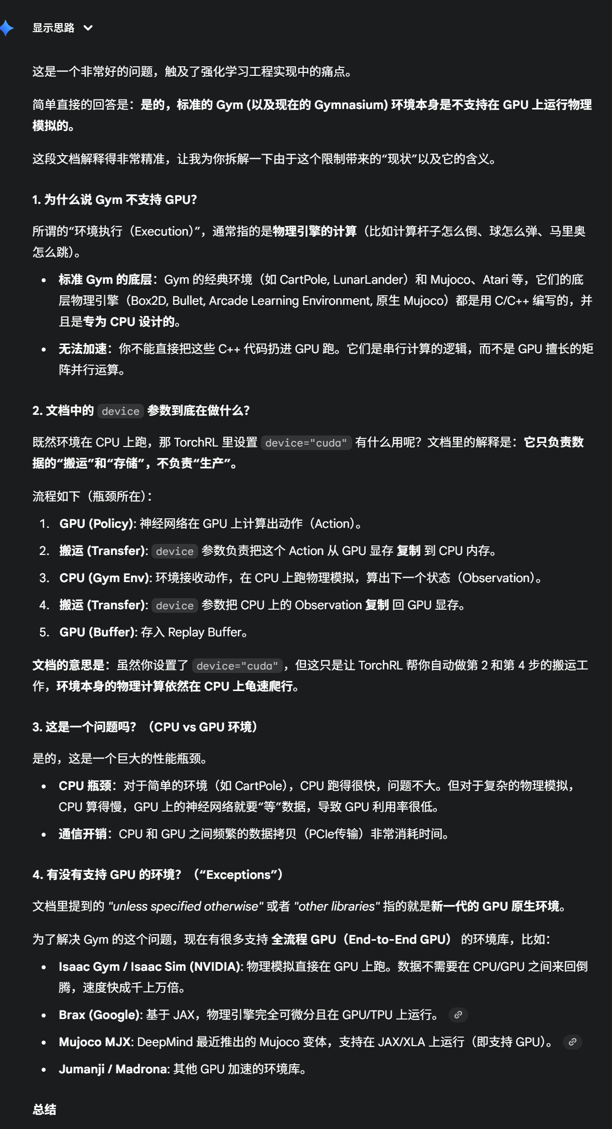
总结
你看到的这段话是在告诉你: "别指望设个 cuda 就能加速 Gym 的物理计算,它还是得回 CPU 跑。除非你用的是 Isaac Gym 或 Brax 这种专门的 GPU 环境库。"