【漫话机器学习系列】199.过拟合 vs 欠拟合（Overfit vs Underfit）

机器学习核心问题：过拟合 vs 欠拟合 ------ 原理详解 + 公式推导 + Python实操

图示作者：Chris Albon

1. 什么是拟合（Fit）？

拟合（Fit）是指模型对数据的学习效果。

理想目标：

在训练集上效果好

在测试集上效果也好

不复杂、不简单，恰到好处

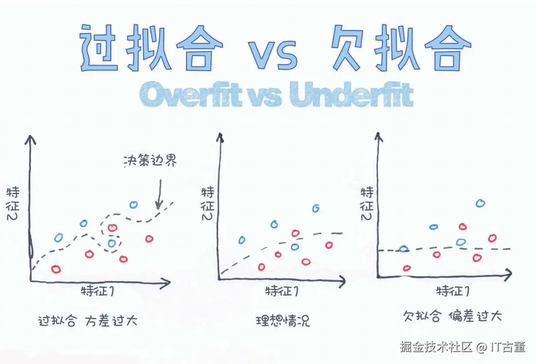
2. 什么是过拟合（Overfitting）？

定义

过拟合是指模型在训练集上表现很好，但在测试集或新数据上效果很差。模型学到了"噪声"或"异常值"的特征。

特征

特征	表现
方差很大	对数据过度敏感
决策边界复杂	曲折、震荡
泛化能力差	新数据易失败

图示（来自图片左侧）

markdown 复制代码

特征2 ↑
       ● ○   ○
        ○ ○
    ○ ● ● ○  ← 决策边界很曲折
特征1 →

3. 什么是欠拟合（Underfitting）？

定义

欠拟合是指模型太简单，无法捕捉数据的有效规律，无论在训练集还是测试集上效果都不好。

特征

特征	表现
偏差很大	无法拟合数据规律
决策边界简单	接近直线
泛化能力弱	无法有效学习

图示（来自图片右侧）

markdown 复制代码

特征2 ↑
       ● ○   ○
        ○ ○
    ○ ● ● ○  ← 决策边界几乎是直线
特征1 →

4. 理想拟合（Best Fit）

状态

偏差（Bias）适中
方差（Variance）适中
决策边界恰好捕捉规律
泛化能力强

图示（图片中间）

markdown 复制代码

特征2 ↑
       ● ○   ○
        ○ ○
    ○ ● ● ○  ← 决策边界刚刚好
特征1 →

5. 数学公式：偏差-方差分解（Bias-Variance Tradeoff）

理论公式

机器学习期望误差可以分解为：

<math xmlns="http://www.w3.org/1998/Math/MathML"> E [ ( y − f ^ ( x ) ) 2 ] = B i a s 2 [ f ^ ( x ) ] + V a r i a n c e [ f ^ ( x ) ] + I r r e d u c i b l e E r r o r E[(y - \hat{f}(x))^2] = Bias^2[\hat{f}(x)] + Variance[\hat{f}(x)] + Irreducible\ Error </math>E[(y−f^(x))2]=Bias2[f^(x)]+Variance[f^(x)]+Irreducible Error

名称	含义
Bias	偏差，模型简单
Variance	方差，模型敏感
Irreducible Error	无法消除的随机误差

6. Python实操示例

构造数据

python 复制代码

import numpy as np
import matplotlib.pyplot as plt
from sklearn.model_selection import train_test_split
from sklearn.preprocessing import PolynomialFeatures
from sklearn.linear_model import LinearRegression
from sklearn.metrics import mean_squared_error

# 真实函数
def true_func(x):
    return np.sin(2 * np.pi * x)

np.random.seed(0)
x = np.sort(np.random.rand(30))
y = true_func(x) + np.random.normal(scale=0.3, size=x.shape)

x_train, x_test, y_train, y_test = train_test_split(x, y, test_size=0.3)

欠拟合（低阶多项式）

scss 复制代码

poly1 = PolynomialFeatures(degree=1)
x1_train = poly1.fit_transform(x_train.reshape(-1, 1))
x1_test = poly1.transform(x_test.reshape(-1, 1))

model1 = LinearRegression().fit(x1_train, y_train)
print('欠拟合 MSE:', mean_squared_error(y_test, model1.predict(x1_test)))

yaml 复制代码

欠拟合 MSE: 0.418206083278207

过拟合（高阶多项式）

scss 复制代码

poly15 = PolynomialFeatures(degree=15)
x15_train = poly15.fit_transform(x_train.reshape(-1, 1))
x15_test = poly15.transform(x_test.reshape(-1, 1))

model15 = LinearRegression().fit(x15_train, y_train)
print('过拟合 MSE:', mean_squared_error(y_test, model15.predict(x15_test)))

yaml 复制代码

过拟合 MSE: 2.732472745353921

理想情况（适中阶）

scss 复制代码

poly4 = PolynomialFeatures(degree=4)
x4_train = poly4.fit_transform(x_train.reshape(-1, 1))
x4_test = poly4.transform(x_test.reshape(-1, 1))

model4 = LinearRegression().fit(x4_train, y_train)
print('理想拟合 MSE:', mean_squared_error(y_test, model4.predict(x4_test)))

yaml 复制代码

理想拟合 MSE: 0.1546713133312227

7. 如何避免过拟合与欠拟合？

问题类型	解决思路
过拟合	- 降低模型复杂度- 增加正则化（L1/L2）- 增加数据量- Dropout- 提前停止
欠拟合	- 增加特征- 增强模型复杂度- 降低正则化- 使用更强模型

8. 可视化偏差-方差关系（效果示意）

css 复制代码

import numpy as np
import matplotlib.pyplot as plt
from sklearn.model_selection import train_test_split
from sklearn.preprocessing import PolynomialFeatures
from sklearn.linear_model import LinearRegression
from sklearn.metrics import mean_squared_error

# 真实函数
def true_func(x):
    return np.sin(2 * np.pi * x)

np.random.seed(0)
x = np.sort(np.random.rand(30))
y = true_func(x) + np.random.normal(scale=0.3, size=x.shape)

x_train, x_test, y_train, y_test = train_test_split(x, y, test_size=0.3)

complexity = np.arange(1, 15)
train_errors = []
test_errors = []

for d in complexity:
    poly = PolynomialFeatures(degree=d)
    x_tr = poly.fit_transform(x_train.reshape(-1, 1))
    x_te = poly.transform(x_test.reshape(-1, 1))

    model = LinearRegression().fit(x_tr, y_train)
    train_errors.append(mean_squared_error(y_train, model.predict(x_tr)))
    test_errors.append(mean_squared_error(y_test, model.predict(x_te)))

plt.plot(complexity, train_errors, label='Train Error')
plt.plot(complexity, test_errors, label='Test Error')
plt.xlabel('Model Complexity (degree)')
plt.ylabel('MSE')
plt.legend()
plt.show()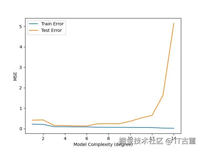

9. 总结

项目	过拟合	欠拟合
决策边界	复杂	简单
偏差Bias	低	高
方差Variance	高	低
表现	训练好，测试差	训练差，测试差

10. 最佳实践

寻找偏差和方差的平衡，是机器学习调参的艺术。

合理的特征工程 + 模型复杂度控制 + 正则化技术，是最佳组合。

如果你觉得这篇文章有帮助，欢迎点赞收藏~