逻辑回归——银行案例（有参数，无处理，下采样，过采样）

评价方式

混淆矩阵：

假设要对 15 个人预测是否患病，使用 1 表示患病，使用 0 表示正常。预测结果如下：

预测值	1	1	1	1	1	0	0	0	0	0	1	1	1	0	1
真实值	0	1	1	0	1	1	0	0	1	0	1	0	1	0	0

\	预测值 = 1	预测值 = 0
真实值 = 1	5	2
真实值 = 0	4	4

评价方式

混淆矩阵：

/	预测值 = 1	预测值 = 0
真实值 = 1	5	2
真实值 = 0	4	4

/	预测值 = 1	预测值 = 0
真实值 = 1	TP	FN
真实值 = 0	FP	TN

TP（True Positive） :5

FP（False Positive） :4

FN（False Negative） :2

TN（True Negative） :4

Accuracy（准确率）：

accuracy = (TP+TN)/(TP+TN+FP+FN)

准确率不一定能完美的表达任何场景

精确率（Precision）的定义公式

公式为

precision=TP/(TP+FP)

recall(召回率)

TP/(TP+FN)

真实值为 1，我预测对了多少个？？

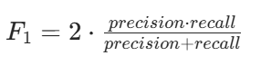
F1-score（F1 值）：

正则化惩罚

目的：
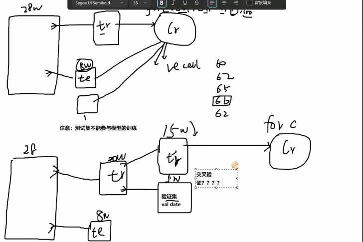
防止过拟合。实体信息是对**模型过拟合**的一种通俗解释：模型过拟合指模型在训练数据（自测）上表现好，但在新的测试数据上效果很差 ，因过度学习训练数据细节（含噪声、异常），缺乏对真实规律的泛化能力 。

概念：

Minimize your error while regularizing your parameters。

规则化参数的同时最小化误差。

像这样的情况两个最低点该如何选择

输入为：x = [1,1,1,1] 现有 2 种不同的权重值，

y = θ₀ + θ₁x₁ + θ₂x₂ + θ₃x₃ + θ₄x₄

输入为：x = [1,1,1,1] 现有 2 种不同的权重值，

w₁ = [1,0,0,0] ------x = [1,1,1,1]------>y = θ₀ + θ₁x₁ + θ₂x₂ + θ₃x₃ + θ₄x₄--y '= 1 + 1 + 0 + 0 + 0 = 2

w₂ = [0.25,0.25,0.25,0.25]-x = [1,1,1,1]--->y′′=1+41​×4=2

惩罚第一种情况，极值点不能只有一个特征

带正则化项的均方差损失函数

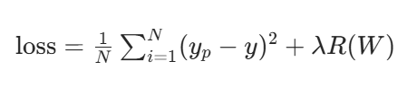
λR(W)：正则化惩罚项

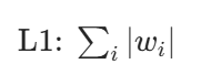
L1,L2是R（W）的，w₁ = [1,0,0,0]代入W即可，发现w₁>w₂,因为要求最小值所以要选w2

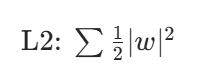
+式子（L2）

原来是这个式子求他的梯度下降 ，像这样的式子加个式子就是正则惩罚项为的约束 θ过于极端化

，也会避开我们刚刚求的第一个式子w₁ = [1,0,0,0] ------x = [1,1,1,1]------>y = θ₀ + θ₁x₁ + θ₂x₂ + θ₃x₃ + θ₄x₄--y '= 1 + 1 + 0 + 0 + 0 = 2这个，

参数的影响

• 坐标轴：横轴 "Size of house（房屋面积）"、纵轴 "Price（价格）"

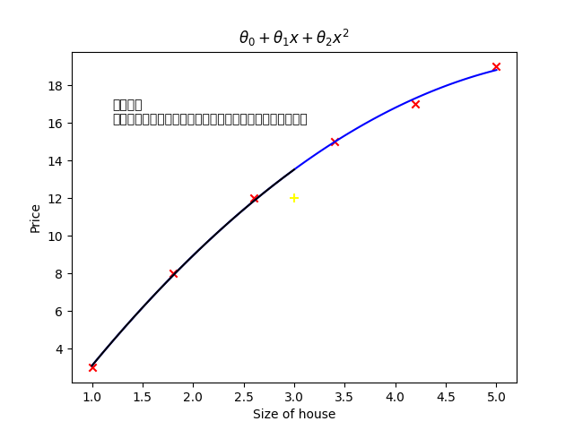
公式；θ₀ + θ₁x + θ₂x²

• 文字说明：简单参数
  虽然不能拟合所有的点，但是可以用来预测，且效果较好。

• 坐标轴：横轴 "Size of house（房屋面积）"、纵轴 "Price（价格）"

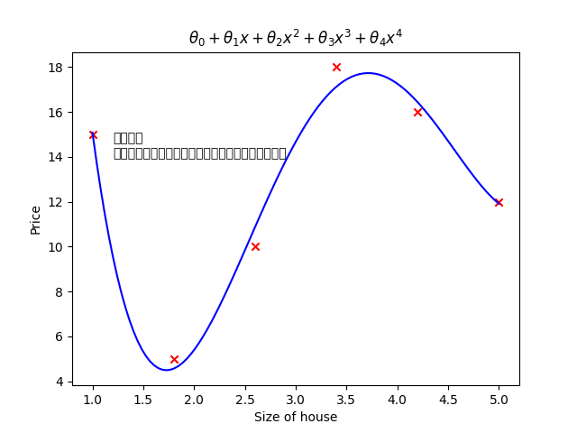
• 公式：θ₀ + θ₁x + θ₂x² + θ₃x³ + θ₄x⁴
• 文字说明：复杂参数
  能够拟合所有的点，但是不能用来预测，效果很差。

二代码

import pandas as pd
import matplotlib.pyplot as plt
from pylab import mpl
import numpy as np

# 绘制可视化混淆矩阵
def cm_plot(y, yp):
    from sklearn.metrics import confusion_matrix
    import matplotlib.pyplot as plt

    cm = confusion_matrix(y, yp)
    plt.matshow(cm, cmap=plt.cm.Blues)
    plt.colorbar()

    for x in range(len(cm)):
        for y in range(len(cm)):
            plt.annotate(cm[x, y], xy=(y, x), horizontalalignment='center',
                         verticalalignment='center')
            plt.ylabel('True label')
            plt.xlabel('Predicted label')
    return plt

"""第一步：数据预处理"""
data = pd.read_csv(r"./creditcard.csv")

"""绘制图形，查看正负样本个数"""
# mpl.rcParams['font.sans-serif'] = ['Microsoft YaHei']
# mpl.rcParams['axes.unicode_minus'] = False
#
# labels_count = pd.value_counts(data['Class'])#0有多少个数据，1有多个数据
# plt.title("正负例样本数")
# plt.xlabel("类别")
# plt.ylabel("频数")
# labels_count.plot(kind='bar')
# plt.show()

"""数据标准化：Z标准化"""
from sklearn.preprocessing import StandardScaler

scaler = StandardScaler()
a = data[['Amount']]#返回dataframe数据，而不是series。[]第一个是选谁[]第二个是以二维的形式返回
data['Amount'] = scaler.fit_transform(data[['Amount']])

data = data.drop(['Time'],axis=1)#删除无用列

"""训练集使用下采样数据,测试集使用原始数据进行预测"""
from sklearn.model_selection import train_test_split#对数据集进行切分，训练数据集+测试数据集

#对下采样数据划分
X = data.drop('Class', axis=1)    #对data_c数据进行划分。
y = data.Class#获取data中的列明为class的数据
x_train, x_test, y_train, y_test = train_test_split(X, y, test_size = 0.3, random_state = 0)

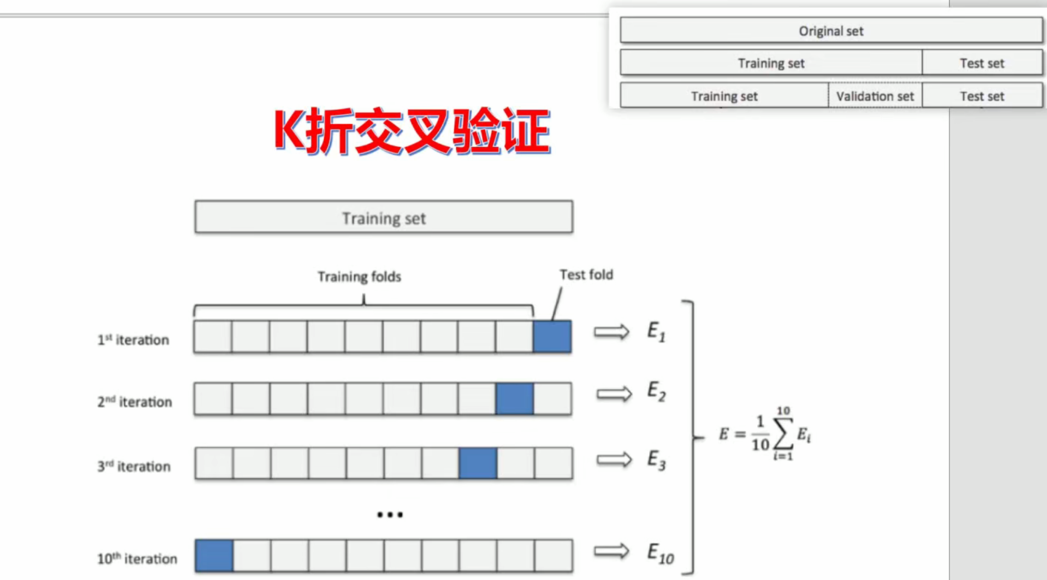
# 执行交叉验证操作
from sklearn.linear_model import LogisticRegression
from sklearn.model_selection import cross_val_score

# 交叉验证选择较优惩罚因子
scores = []
c_param_range = [0.01, 0.1, 1, 10, 100]  # 参数，
for i in c_param_range:  # 第1词循环的时候C=0.01，5个逻辑回归模型
    lr = LogisticRegression(C=i, penalty='l2', solver='lbfgs', max_iter=1000)  # 怎么均衡的来判断模型好不好，
    score = cross_val_score(lr, x_train, y_train, cv=8, scoring='recall')  # 交叉验证。
    # scoring:可选"accuracy"（精度）、recall（召回率）、roc_auc（roc值）、neg_mean_squared_error（均方误差）、
    score_mean = sum(score) / len(score)  # 交叉验证后的值召回率
    scores.append(score_mean)  # 里面保存了所有的交叉验证召回率
    print(score_mean)  # 将不同的c参数分别传入模型，分别看看哪个模型效果更好，我们选c

#
best_c = c_param_range[np.argmax(scores)]#寻找到scores中最大值的对应的C参数
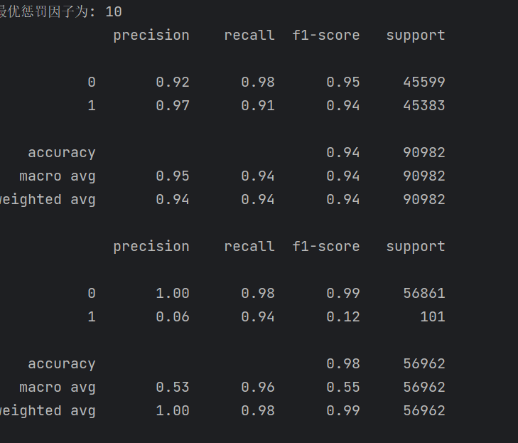
print(".......最优惩罚因子为: {}".format(best_c)) #
# """建立最优模型"""
lr = LogisticRegression(C = best_c, penalty = 'l2', max_iter = 1000)#c=【100，10，1，0.1，0.01】
lr.fit(x_train, y_train)    #fit训练集进行，深度学习。

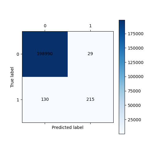
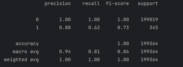
# # #绘制混淆矩阵
from sklearn import metrics#函数是专门用来做测试的。
train_predicted = lr.predict(x_train)#测试机进行
print(metrics.classification_report(y_train, train_predicted))#自测
cm_plot(y_train, train_predicted).show()

# 交叉验证选择较优惩罚因子
scores = []
c_param_range = [0.01, 0.1, 1, 10, 100]  # 参数，
for i in c_param_range:  # 第1词循环的时候C=0.01，5个逻辑回归模型
    lr = LogisticRegression(C=i, penalty='l2', solver='lbfgs', max_iter=1000)  # 怎么均衡的来判断模型好不好，
    score = cross_val_score(lr, x_train, y_train, cv=8, scoring='recall')  # 交叉验证。
    # scoring:可选"accuracy"（精度）、recall（召回率）、roc_auc（roc值）、neg_mean_squared_error（均方误差）、
    score_mean = sum(score) / len(score)  # 交叉验证后的值召回率
    scores.append(score_mean)  # 里面保存了所有的交叉验证召回率
    print(score_mean)  # 将不同的c参数分别传入模型，分别看看哪个模型效果更好，我们选c

#
best_c = c_param_range[np.argmax(scores)]#寻找到scores中最大值的对应的C参数
print(".......最优惩罚因子为: {}".format(best_c)) #
# """建立最优模型"""
lr = LogisticRegression(C = best_c, penalty = 'l2', max_iter = 1000)#c=【100，10，1，0.1，0.01】
lr.fit(x_train, y_train)    #fit训练集进行，深度学习。

C的数据集该如何选择

# 执行交叉验证操作
from sklearn.linear_model import LogisticRegression
from sklearn.model_selection import cross_val_score

交叉验证

图

如果要提高recall那么就要提高阈值

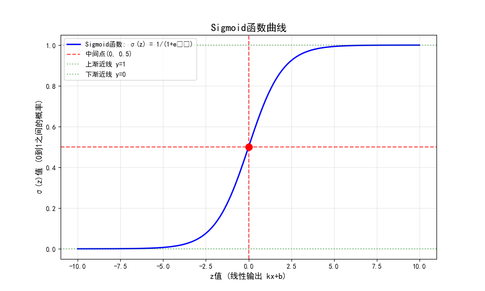
这个十字可以看成x轴和y轴点就是可以调节阈值的调高那么会靠近y轴那么会大幅度提高正确率，

hresholds = [0.1,0.2,0.3,0.4,0.5,0.6,0.7,0.8,0.9]
recalls = []
for i in thresholds:
    y_predict_proba = lr.predict_proba(x_test)

    y_predict_proba = pd.DataFrame(y_predict_proba)
    y_predict_proba = y_predict_proba.drop([0],axis=1)
    y_predict_proba[y_predict_proba[1] > i] = 1   # 当预测的概率大于i，0.1，0.2，
    y_predict_proba[y_predict_proba[1] <= i] = 0  # 当预测的概率小于等于i  预测的标
    # y_pred = (y_predict_proba > i).astype(int)
    # cm_plot(y_test, y_predict_proba[1]).show()
    recall = metrics.recall_score(y_test, y_predict_proba[1])
    recalls.append(recall)
    print("{} Recall metric in the testing dataset: {:.3f}".format(i,recall))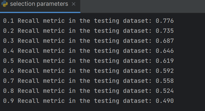

正确率还是不够所以我们开始调整数据集，原有的数据集是不均衡的

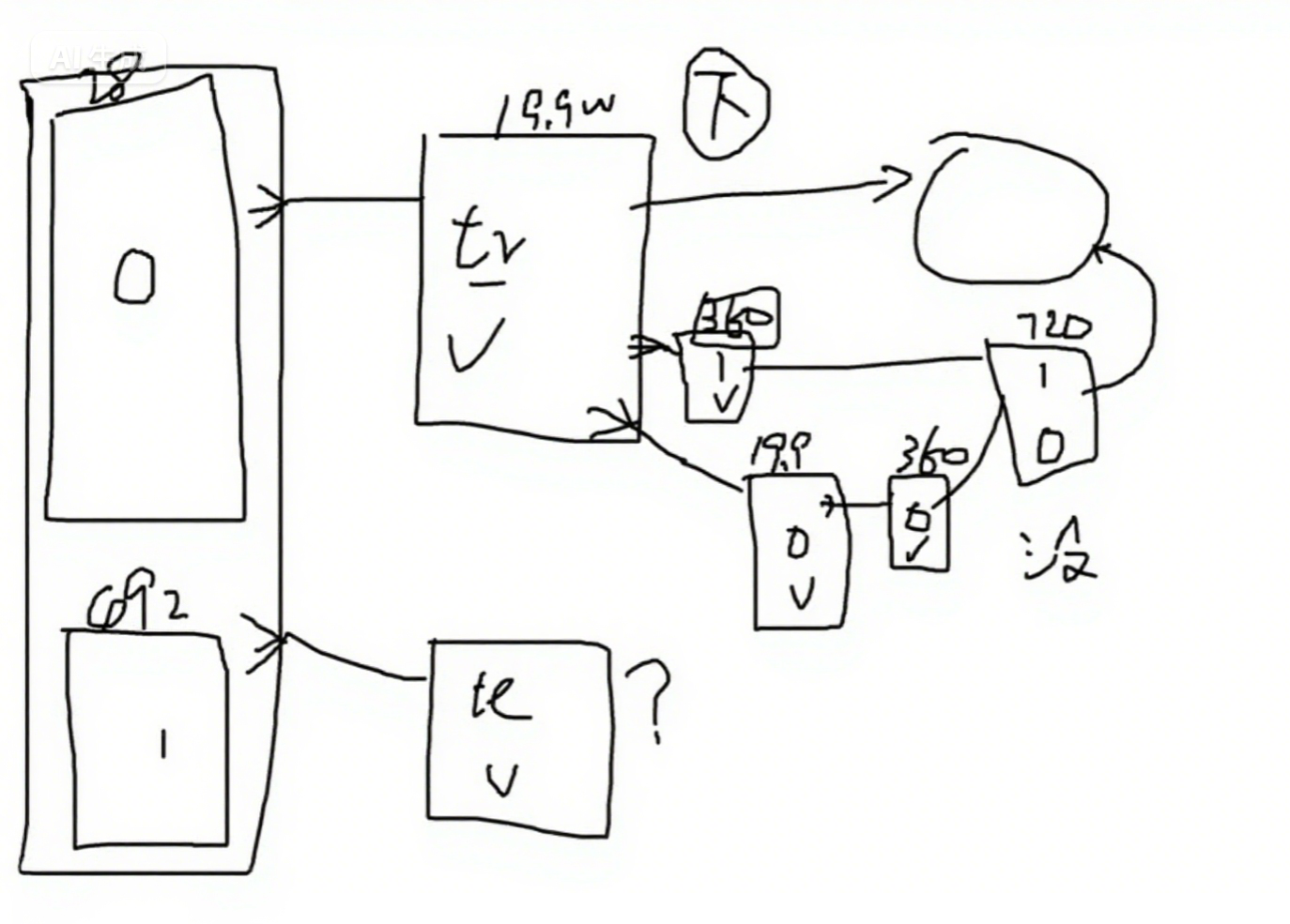
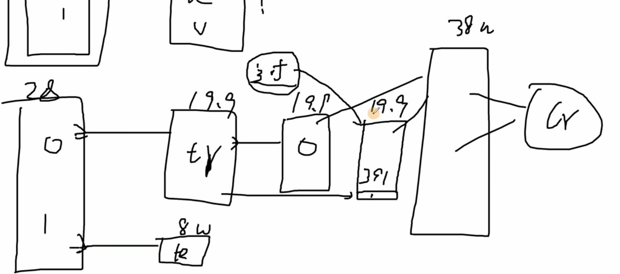
下采样这个图的逻辑走

import pandas as pd
import matplotlib.pyplot as plt
from pylab import mpl
import numpy as np
from sklearn.model_selection import train_test_split, cross_val_score
from sklearn.linear_model import LogisticRegression
from sklearn import metrics
from sklearn.preprocessing import StandardScaler

# 第一步：数据预处理
data = pd.read_csv(r"./creditcard.csv")

# 数据标准化：Z标准化
scaler = StandardScaler()
a = data[['Amount']]  # 返回DataFrame数据，而不是Series
data['Amount'] = scaler.fit_transform(data[['Amount']])
data = data.drop(['Time'], axis=1)  # 删除无用列

# 对原始数据集进行切分，用于后期的测试
X_whole = data.drop('Class', axis=1)
y_whole = data.Class
x_train_w, x_test_w, y_train_w, y_test_w = train_test_split(X_whole, y_whole, test_size=0.2, random_state=0)

# 构建训练集数据
x_train_w['Class'] = y_train_w
data_train = x_train_w

# 下采样解决样本不均衡问题
positive_eg = data_train[data_train['Class'] == 0]  # 获取正例样本
negative_eg = data_train[data_train['Class'] == 1]  # 获取负例样本
positive_eg = positive_eg.sample(len(negative_eg))  # 对正例样本下采样
data_c = pd.concat([positive_eg, negative_eg])  # 拼接数据

# 训练集使用下采样数据，测试集使用原始数据进行预测
X = data_c.drop('Class', axis=1)
y = data_c.Class
x_train, x_test, y_train, y_test = train_test_split(X, y, test_size=0.3, random_state=0)

scores = []
c_param_range = [0.01,0.1,1,10,100]#交叉验证选择较优惩罚因子
for i in c_param_range:
    lr = LogisticRegression(C = i, penalty = 'l2', solver='lbfgs', max_iter=1000)
    score = cross_val_score(lr, X, y, cv=5,scoring='recall')
    score_mean = sum(score)/len(score)
    scores.append(score_mean)
    print(score_mean)

best_c = c_param_range[np.argmax(scores)]#寻找到scores中最大值的对应的C参数
# 建立最优模型
lr = LogisticRegression(C=best_c, penalty='l2', max_iter=1000)
lr.fit(X, y)
'''小训练集数据进行自测'''
train_predicted = lr.predict(X)
print(metrics.classification_report(y, train_predicted))#小数据集的训练数据集

"""使用测试集数据进行测试【大测试集】"""
test_predicted_big = lr.predict(x_test_w)#大数据测试数据集来进行预测
print(metrics.classification_report(y_test_w, test_predicted_big))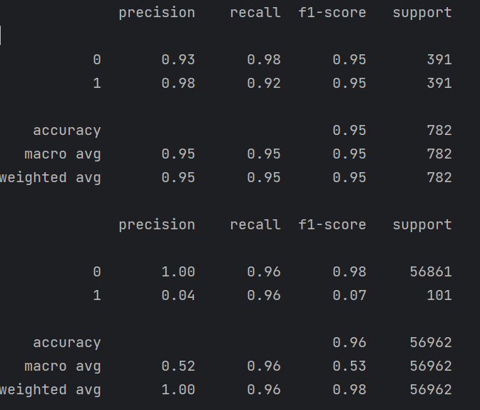

结果也没有出现过拟合

过采样

那什么样的方法可以过拟合呢

过采样

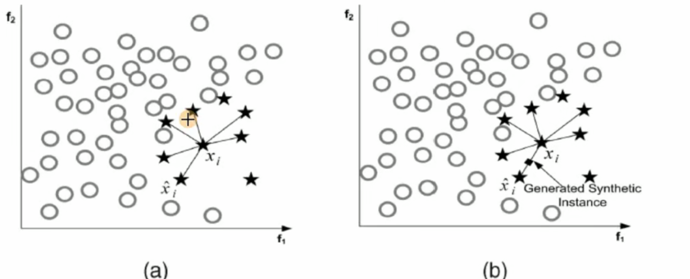
SMOTE 算法：

SMOTE（Synthetic Minority Oversampling Technique）即合成少数类过采样技术，它是基于随机过采样算法的一种改进方案，SMOTE 算法的基本思想是对少数类样本进行分析并根据少数类样本人工合成新样本添加到数据集中。

文字内容：

过采样

SMOTE 算法：

1. 对于少数类中每一个样本 x，以欧氏距离为标准计算它到少数类样本集 Sₘᵢₙ中所有样本的距离，得到其 k 近邻。
2. 根据样本不平衡比例设置一个采样比例以确定采样倍率 N，对于每一个少数类样本 x，从其 k 近邻中随机选择若干个样本，假设选择的近邻为 xn。
3. 对于每一个随机选出的近邻 xn，分别与原样本按照如下的公式构建新的样本
   𝑥ₙₑ𝑤 = 𝑥 + 𝑟𝑎𝑛𝑑(0,1) ∗ |𝑥 − 𝑥𝑛|

import pandas as pd
import numpy as np
import matplotlib.pyplot as plt
from pylab import mpl
import time
from sklearn.model_selection import train_test_split, cross_val_score
from sklearn.linear_model import LogisticRegression
from sklearn import metrics
from sklearn.preprocessing import StandardScaler
from imblearn.over_sampling import SMOTE

# 第一步：数据预处理
data = pd.read_csv(r".\creditcard.csv", encoding='utf8', engine='python')

# 数据标准化：Z标准化
scaler = StandardScaler()
data['Amount'] = scaler.fit_transform(data[['Amount']])
data = data.drop(['Time'], axis=1)  # 删除无用列

# 切分原始数据集
X_whole = data.drop('Class', axis=1)
y_whole = data.Class
x_train_w, x_test_w, y_train_w, y_test_w = train_test_split(X_whole, y_whole, test_size=0.2, random_state=0)

# 进行过采样操作
oversampler = SMOTE(random_state=0)
os_x_train, os_y_train = oversampler.fit_resample(x_train_w, y_train_w)

# 拟合数据集（对过采样后的数据再切分）
os_x_train_w, os_x_test_w, os_y_train_w, os_y_test_w = train_test_split(os_x_train, os_y_train, test_size=0.2, random_state=0)

# 交叉验证选择较优惩罚因子
scores = []
c_param_range = [0.01, 0.1, 1, 10, 100]
z = 1
for i in c_param_range:
    start_time = time.time()
    lr = LogisticRegression(C=i, penalty='l2', solver='lbfgs', max_iter=1000)
    score = cross_val_score(lr, os_x_train_w, os_y_train_w, cv=5, scoring='recall')
    score_mean = sum(score) / len(score)
    scores.append(score_mean)
    end_time = time.time()
    print(f"第{z}次...")
    print(f"time spend:{end_time - start_time:.2f}")
    print(f"recall:{score_mean}")
    z += 1

# 确定最优惩罚因子并建立最优模型
best_c = c_param_range[np.argmax(scores)]
print(f"最优惩罚因子为: {best_c}")
lr = LogisticRegression(C=best_c, penalty='l2', solver='lbfgs', max_iter=1000)
lr.fit(os_x_train_w, os_y_train_w)

# 模型评估（训练集预测 & 分类报告输出）
train_predicted = lr.predict(os_x_test_w)
print(metrics.classification_report(os_y_test_w, train_predicted))
#训练集预测概率【小数据集】  原始 28w
test_predicted = lr.predict(x_test_w)
print(metrics.classification_report(y_test_w, test_predicted))