周志华院士西瓜书实战（一）线性规划+多项式回归+逻辑回归+决策树

目录

[1. 线性规划](#1. 线性规划)

[2. 多项式回归](#2. 多项式回归)

[3. 逻辑回归手写数字](#3. 逻辑回归手写数字)

[4. Pytorch MNIST](#4. Pytorch MNIST)

[5. 决策树](#5. 决策树)

---

1. 线性规划

先生成 Y=1.5X+0.2+ε 的（X,Y）训练数据 两个长度为30

import numpy as np
import matplotlib.pyplot as plt 

def true_fun(X): # 这是我们设定的真实函数，即ground truth的模型
    return 1.5*X + 0.2

np.random.seed(0) # 设置随机种子
n_samples = 30 # 设置采样数据点的个数

'''生成随机数据作为训练集，并且加一些噪声'''
X_train = np.sort(np.random.rand(n_samples)) 
y_train = (true_fun(X_train) + np.random.randn(n_samples) * 0.05).reshape(n_samples,1)

sklearn中线性回归模型 其中X_train[:,np.newaxis] 是把长度30的向量 转化为二维的(30,1)

from sklearn.linear_model import LinearRegression # 导入线性回归模型
model = LinearRegression() # 定义模型
model.fit(X_train[:,np.newaxis], y_train) # 训练模型
print("输出参数w：",model.coef_) # 输出模型参数w
print("输出参数b：",model.intercept_) # 输出参数b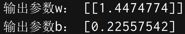

可视化绘图一下 用 linspace 生成(0,1))之间100个点 分别输出散点图；原线性；拟合线性

X_test = np.linspace(0, 1, 100)
plt.plot(X_test, model.predict(X_test[:, np.newaxis]), label="Model")
plt.plot(X_test, true_fun(X_test), label="True function")
plt.scatter(X_train,y_train) # 画出训练集的点
plt.legend(loc="best")
plt.show()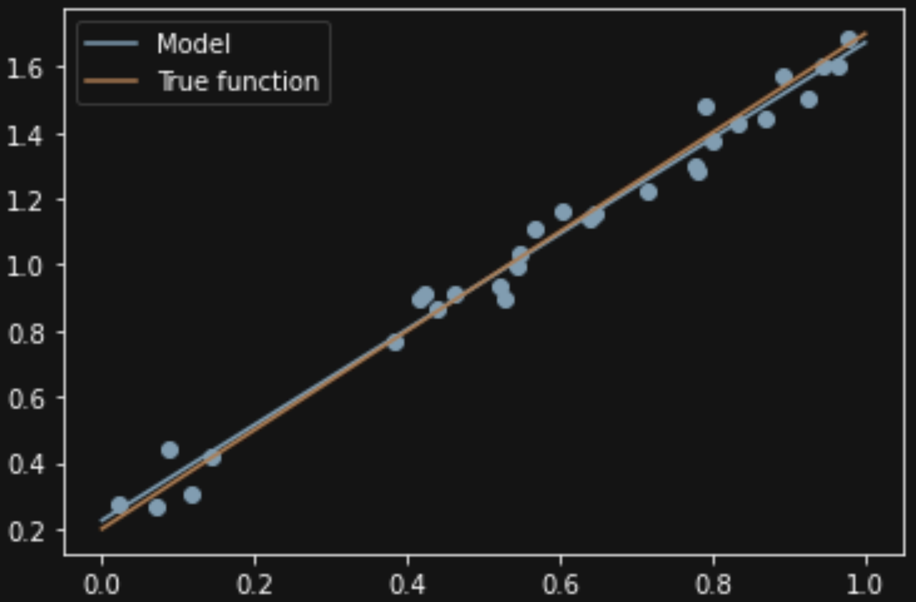

2. 多项式回归

导入多项式和交叉验证的库 原函数为余弦函数

import numpy as np
import matplotlib.pyplot as plt
from sklearn.pipeline import Pipeline
from sklearn.preprocessing import PolynomialFeatures # 导入能够计算多项式特征的类
from sklearn.linear_model import LinearRegression
from sklearn.model_selection import cross_val_score

def true_fun(X): # 这是我们设定的真实函数，即ground truth的模型
    return np.cos(1.5 * np.pi * X)
np.random.seed(0)
n_samples = 30 # 设置随机种子

X = np.sort(np.random.rand(n_samples)) 
y = true_fun(X) + np.random.randn(n_samples) * 0.1

3种多项式 polynomial_features构建x的多次方 再拼接到线性回归

degrees = [1, 4, 15] # 多项式最高次
plt.figure(figsize=(14, 5))
for i in range(len(degrees)):
    ax = plt.subplot(1, len(degrees), i + 1)
    plt.setp(ax, xticks=(), yticks=())
    polynomial_features = PolynomialFeatures(degree=degrees[i],
                                             include_bias=False)
    linear_regression = LinearRegression()
    pipeline = Pipeline([("polynomial_features", polynomial_features),
                         ("linear_regression", linear_regression)]) # 使用pipline串联模型
    pipeline.fit(X[:, np.newaxis], y)
    
    scores = cross_val_score(pipeline, X[:, np.newaxis], y,scoring="neg_mean_squared_error", cv=10) # 使用交叉验证

作图发现1欠拟合 15过拟合 4刚好

    X_test = np.linspace(0, 1, 100)
    plt.plot(X_test, pipeline.predict(X_test[:, np.newaxis]), label="Model")
    plt.plot(X_test, true_fun(X_test), label="True function")
    plt.scatter(X, y, edgecolor='b', s=20, label="Samples")
    plt.xlabel("x")
    plt.ylabel("y")
    plt.xlim((0, 1))
    plt.ylim((-2, 2))
    plt.legend(loc="best")
    plt.title("Degree {}\nMSE = {:.2e}(+/- {:.2e})".format(
        degrees[i], -scores.mean(), scores.std()))
plt.show()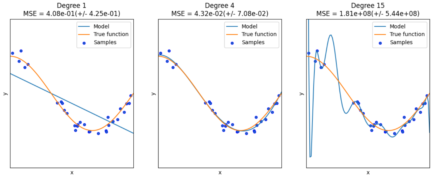

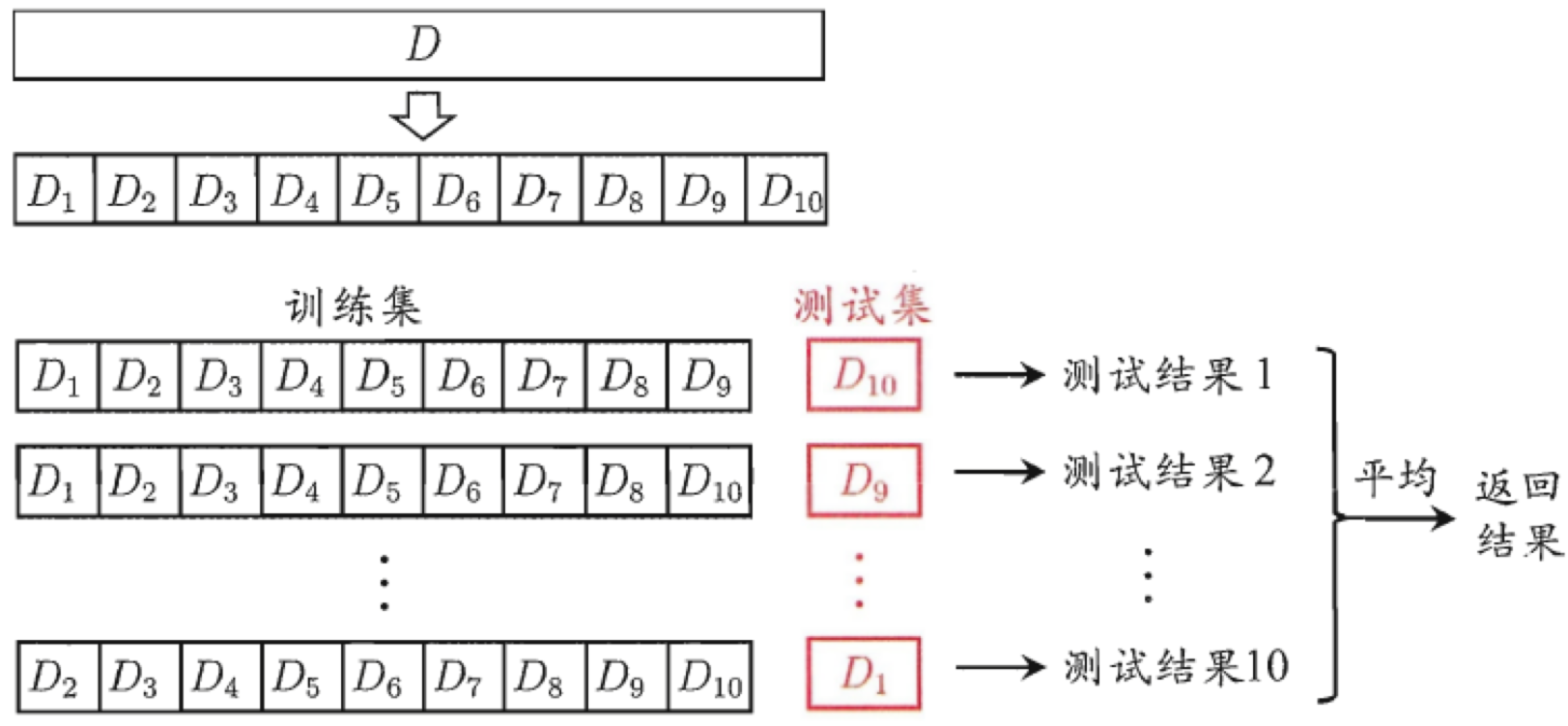
10折交叉验证（数据分为10份，轮流用9份训练、1份验证，重复10次）

3. 逻辑回归手写数字

MNIST数据集每张图像是 28*28的 前60000张训练 后10000测试

LogisticRegression 使用L1正则化 选择求解器；训练容忍率（越小 训练久精度高）

对于train数据 fit拟合一下；对于test 计算误差值

import numpy as np
from sklearn.datasets import fetch_openml
from sklearn.linear_model import LogisticRegression

# 数据
mnist = fetch_openml('mnist_784')
X, y = mnist['data'], mnist['target']
X_train = np.array(X[:60000], dtype=float)
y_train = np.array(y[:60000], dtype=float)
X_test = np.array(X[60000:], dtype=float)
y_test = np.array(y[60000:], dtype=float)

print(X_train.shape)
print(y_train.shape)
print(X_test.shape)
print(y_test.shape)

clf = LogisticRegression(penalty="l1", solver="saga", tol=0.1)
clf.fit(X_train, y_train)
score = clf.score(X_test, y_test)
print("Test score with L1 penalty: %.4f" % score)

4. Pytorch MNIST

在上上层路径加载数据集 并转化为Tensor形式

from torch.utils.data import DataLoader
from torchvision import datasets
import torchvision
import torchvision.transforms as transforms
import matplotlib.pyplot as plt
from sklearn.linear_model import LogisticRegression
from sklearn.metrics import classification_report
import numpy as np
import sys
from pathlib import Path
p_parent_path = str(Path().absolute().parent.parent)
sys.path.append(p_parent_path)
train_dataset = datasets.MNIST(root = p_parent_path+'/datasets/', train = True,transform = transforms.ToTensor(), download = True)
test_dataset = datasets.MNIST(root = p_parent_path+'/datasets/', train = False,
                               transform = transforms.ToTensor(), download = True)

将图像数据从(60000, 1, 28, 28)转化为array 再转换为(60000, 784)的二维矩阵

batch_size = len(train_dataset)
train_loader = DataLoader(dataset=train_dataset, batch_size=batch_size, shuffle=True)
test_loader = DataLoader(dataset=test_dataset, batch_size=batch_size, shuffle=False)

X_train,y_train = next(iter(train_loader))
X_test,y_test = next(iter(test_loader))

# 合并数据并转换为numpy数组
X_train,y_train = X_train.cpu().numpy(),y_train.cpu().numpy() # tensor转为array形式)
X_test,y_test = X_test.cpu().numpy(),y_test.cpu().numpy() # tensor转为array形式)
X_train = X_train.reshape(X_train.shape[0],784)
X_test = X_test.reshape(X_test.shape[0],784)

使用L-BFGS优化器（拟牛顿法） 设置最大迭代次数为400次 指定多分类问题（multinomial）

model = LogisticRegression(solver='lbfgs', max_iter=400, multi_class='multinomial')
model.fit(X_train, y_train)

# 评估模型
y_pred = model.predict(X_test)
print(classification_report(y_test, y_pred))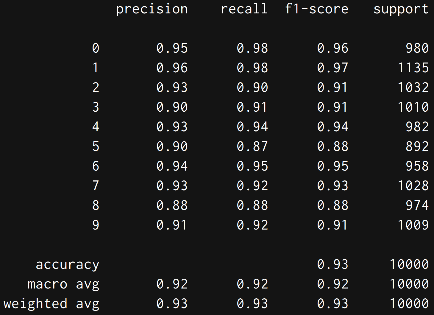

5. 决策树

加载iris数据集 把二维data加载到X 把向量加载到y（并且把0 1 2映射到真实花名）

import pandas as pd
import numpy as np
import matplotlib.pyplot as plt
from sklearn.tree import DecisionTreeClassifier
from sklearn.datasets import load_iris
from sklearn.model_selection import train_test_split
from sklearn import tree

# 加载数据集
data = load_iris()
X = pd.DataFrame(data.data, columns=data.feature_names)
y = pd.Series(data.target).map(dict(zip(np.unique(data.target), data.target_names)))

划分训练-测试集 建立决策树进行fit训练 criterion 可用 'gini' 基尼系数 或 'entropy' 信息增益

X_train, test_x, y_train, test_lab = train_test_split(X,y,test_size = 0.4,random_state = 42)
model = DecisionTreeClassifier(max_depth =3, random_state = 42)
model.fit(X_train, y_train) 

使用 文字/图像 两种方式输出

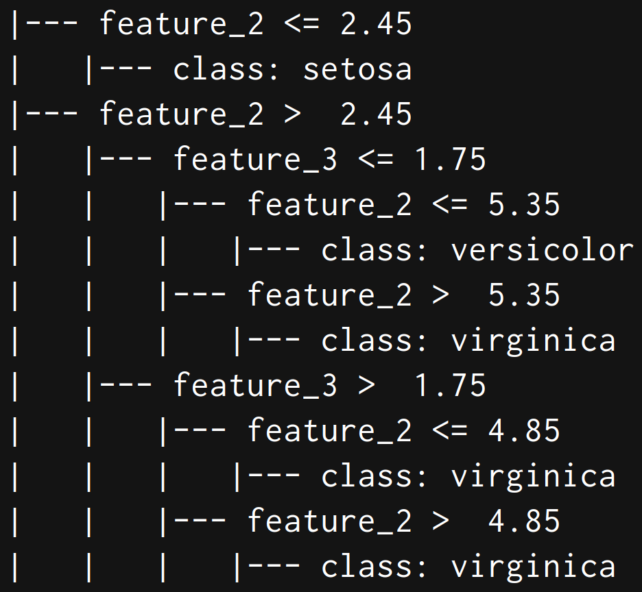
# 以文字形式输出树     
text_representation = tree.export_text(model)
print(text_representation)
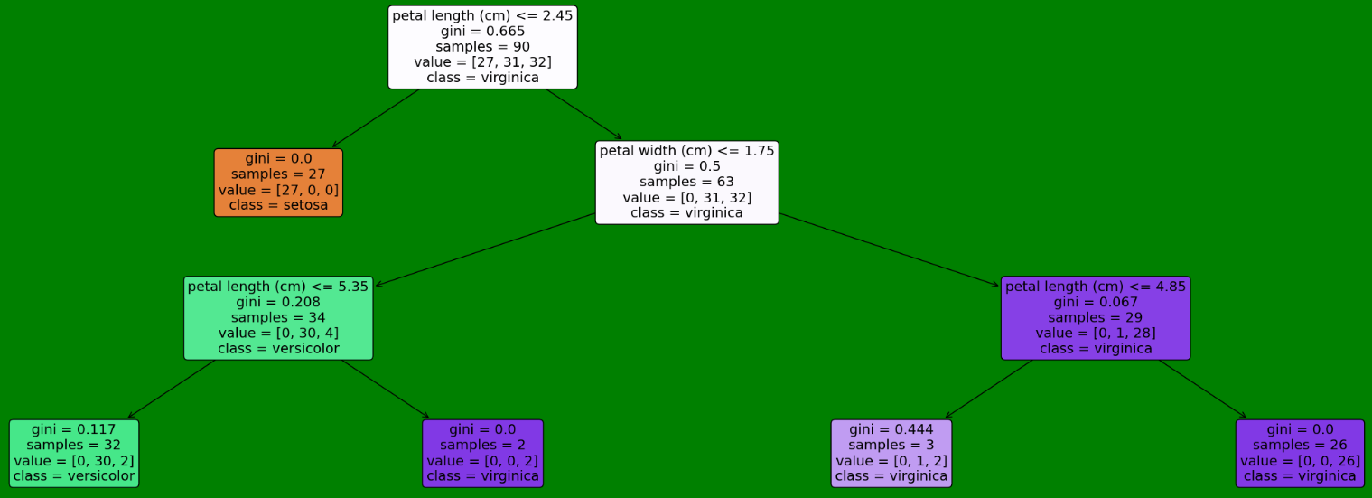
# 用图片画出
plt.figure(figsize=(30,10), facecolor ='g') 
a = tree.plot_tree(model,
                   feature_names = data.feature_names, #特征名
                   class_names = y.unique(), #类名
                   filled = True, #颜色深浅代表纯度
                   fontsize=14)
plt.show()          
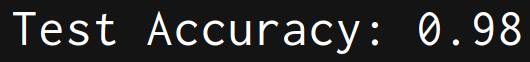
test_acc = model.score(test_x, test_lab)
print(f"\nTest Accuracy: {test_acc:.2f}")