使用sklearn进行多项式拟合（回归模型训练）并可视化展示对比

python 复制代码
# coding=utf-8
import numpy as np
import matplotlib.pyplot as plt
from sklearn.linear_model import LinearRegression
from sklearn.preprocessing import PolynomialFeatures
from sklearn.pipeline import Pipeline
from sklearn.model_selection import train_test_split
from sklearn.metrics import mean_squared_error, r2_score

plt.rcParams['font.sans-serif'] = ['SimHei']  # Windows系统常用，解决中文乱码问题
plt.rcParams['axes.unicode_minus'] = False    # 解决负号显示问题

# 设置随机种子以确保结果可重现
np.random.seed(42)

# 1. 生成示例数据
# 假设我们有两个输入特征和一个输出
n_samples = 200
X = np.random.rand(n_samples, 2) * 10 - 5 # 生成在[-5, 5]范围内的二维特征
# 创建非线性关系：y = x1^2 + 2*x2^2 + x1*x2 + 噪声
y = X[:, 0]**2 + 2*X[:, 1]**2 + X[:, 0]*X[:, 1] + np.random.randn(n_samples) * 1

# 2. 划分训练集和测试集
X_train, X_test, y_train, y_test = train_test_split(X, y, test_size=0.2, random_state=42)

# 3. 创建并训练多项式回归模型
# 创建多项式回归模型管道
model = Pipeline([
    ('poly', PolynomialFeatures(degree=3)), # 3次多项式特征
    ('linear', LinearRegression())
])

# 拟合数据
model.fit(X_train, y_train)

# 4. 进行预测
train_predictions = model.predict(X_train)
test_predictions = model.predict(X_test)

# 5. 评估模型性能
train_mse = mean_squared_error(y_train, train_predictions)
test_mse = mean_squared_error(y_test, test_predictions)
train_r2 = r2_score(y_train, train_predictions)
test_r2 = r2_score(y_test, test_predictions)

print(f"训练集MSE: {train_mse:.4f}")
print(f"测试集MSE: {test_mse:.4f}")
print(f"训练集R: {train_r2:.4f}")
print(f"测试集R: {test_r2:.4f}")

# 6. 可视化结果
# 由于我们的输入是二维的，我们需要选择一个维度来可视化
# 这里我们固定x2=0，展示y与x1的关系
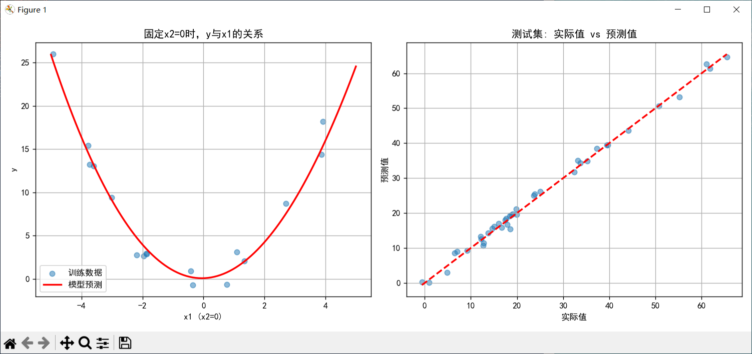
plt.figure(figsize=(12, 5))

# 子图1: 固定x2=0，展示y与x1的关系
plt.subplot(1, 2, 1)
x1_range = np.linspace(-5, 5, 100)
x2_fixed = np.zeros(100) # 固定x2=0
X_plot = np.column_stack((x1_range, x2_fixed))
y_plot = model.predict(X_plot)

# 找出训练集中x2接近0的点
mask = np.abs(X_train[:, 1]) < 0.5
plt.scatter(X_train[mask, 0], y_train[mask], alpha=0.5, label='训练数据')
plt.plot(x1_range, y_plot, 'r-', linewidth=2, label='模型预测')
plt.xlabel('x1 (x2=0)')
plt.ylabel('y')
plt.title('固定x2=0时，y与x1的关系')
plt.legend()
plt.grid(True)

# 子图2: 实际值与预测值的散点图
plt.subplot(1, 2, 2)
plt.scatter(y_test, test_predictions, alpha=0.5)
plt.plot([y_test.min(), y_test.max()], [y_test.min(), y_test.max()], 'r--', linewidth=2)
plt.xlabel('实际值')
plt.ylabel('预测值')
plt.title('测试集: 实际值 vs 预测值')
plt.grid(True)

plt.tight_layout()
plt.show()

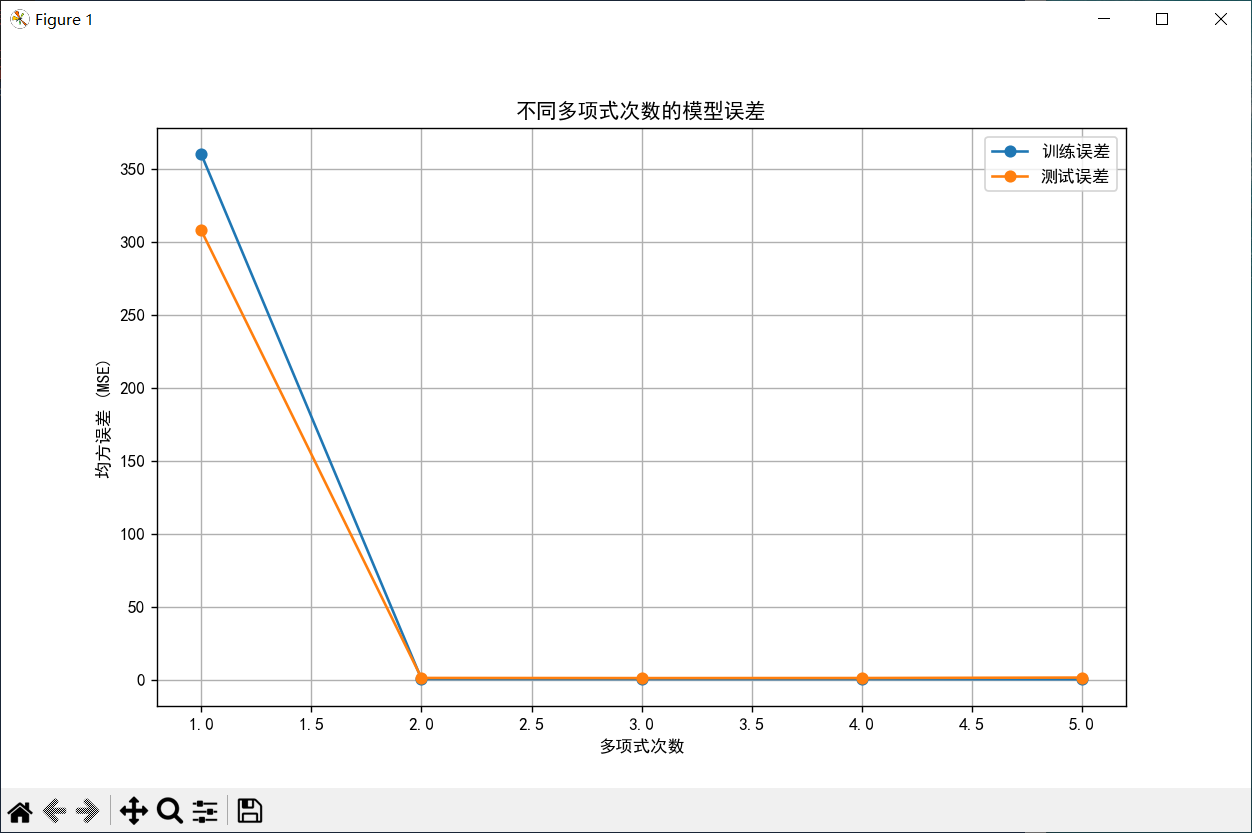
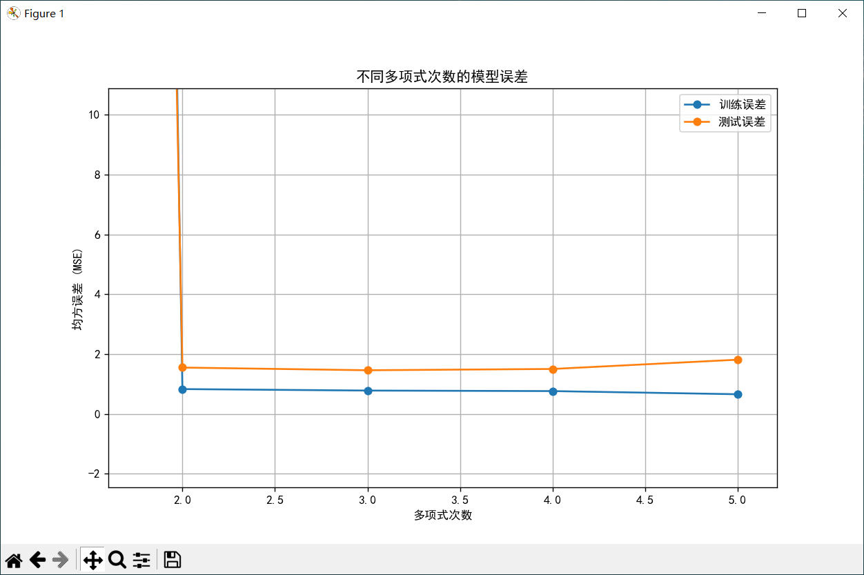
# 7. 探索不同多项式次数的影响
degrees = [1, 2, 3, 4, 5]
train_errors = []
test_errors = []

for degree in degrees:
    # 创建并训练模型
    model = Pipeline([
        ('poly', PolynomialFeatures(degree=degree)),
        ('linear', LinearRegression())
    ])
    model.fit(X_train, y_train)
    
    # 计算误差
    train_pred = model.predict(X_train)
    test_pred = model.predict(X_test)
    train_errors.append(mean_squared_error(y_train, train_pred))
    test_errors.append(mean_squared_error(y_test, test_pred))

# 绘制误差曲线
plt.figure(figsize=(10, 6))
plt.plot(degrees, train_errors, 'o-', label='训练误差')
plt.plot(degrees, test_errors, 'o-', label='测试误差')
plt.xlabel('多项式次数')
plt.ylabel('均方误差 (MSE)')
plt.title('不同多项式次数的模型误差')
plt.legend()
plt.grid(True)
plt.show()

# 8. 查看模型系数
# 获取多项式特征名称
poly_features = model.named_steps['poly'].get_feature_names_out(['x1', 'x2'])
# 获取线性回归系数
coefficients = model.named_steps['linear'].coef_
intercept = model.named_steps['linear'].intercept_

print("\n模型系数:")
print(f"截距: {intercept:.4f}")
for feature, coef in zip(poly_features, coefficients):
    print(f"{feature}: {coef:.4f}")

# 9. 使用模型进行新预测
# 创建一些新数据点进行预测
new_points = np.array([
    [2.0, 1.0], # 点1
    [-3.0, 2.0], # 点2
    [0.0, 0.0] # 点3
])

predictions = model.predict(new_points)
print("\n新数据点的预测:")
for i, (point, pred) in enumerate(zip(new_points, predictions)):
    print(f"点{i+1} {point}: 预测值 = {pred:.4f}")
解决类似的问题，除了上述sklearn库多项式回归的方法，还有支持向量回归（SVR）、随机森林回归、梯度提升回归等方法，以及TensorFlow/Keras/PyTorch的神经网络方法等。
注：以上代码借助Ai生成，并运行通过。