机器人强化学习Ant

机器人强化学习------Ant

从本节起，我们将介绍机器人强化学习，即机器人通过强化学习算法进行自主学习和控制。机器人强化学习是强化学习在机器人领域的应用，是机器人领域的研究热点之一。我们将使用gym中的mujoco库进行机器人强化学习的研究。

MuJoCo（Multi-Joint dynamics with

Contact）是一个物理引擎，用于促进机器人、生物力学、图形和动画以及其他需要快速准确模拟的领域的研究和开发。MuJoCo具有以下特点：

高精度物理模拟：MuJoCo以其高精度的物理模拟能力而著称，能够准确地模拟机器人、生物力学等领域的复杂动力学过程。
广泛的应用领域：MuJoCo不仅被广泛应用于机器人控制优化等研究领域，还可以用于图形和动画的制作，为相关领域的研究和开发提供了强大的工具。

MuJoCo库中包含了多个机器人模型，如Ant、Humanoid、Hopper等。这些模型具有不同的结构和运动方式，可以用于不同的强化学习任务。在本节中，我们将介绍如何使用MuJoCo库中的Ant模型进行强化学习。

Ant模型是一个六足机器人，具有12个自由度。在MuJoCo中，Ant模型被表示为一个包含多个关节和连杆的物理模型。每个关节和连杆都有相应的物理属性，如质量、惯性矩、摩擦系数等。通过控制这些关节的角速度，可以实现对Ant模型的控制。

注意：本文用到了PyTorch库，gym强化学习环境库，需要提前安装。

gym环境安装：https://github.com/Farama-Foundation/Gymnasium
gym环境介绍文档：https://gymnasium.farama.org/environments/classic_control/mountain_car/
pytorch官网：https://pytorch.org/

本文所使用的python版本为3.11.8，其中mujoco环境和open-cv库可通过下方命令安装。（本文所述的强化学习过程最好在linux系统主机中运行）

python 复制代码

%pip install "gymnasium[mujoco]"

python 复制代码

%pip install opencv-python

Step1: Ant游戏简介

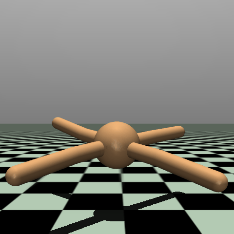
Ant环境基于Schulman、Moritz、Levine、Jordan和Abbeel在《使用广义优势估计的高维连续控制》中介绍的环境。蚂蚁是一个3D机器人，由一个躯干（可自由旋转的身体）和四条腿组成，每条腿有两个身体部分。目标是通过在连接每条腿的两个身体部分和躯干（九个身体部分和八个铰链）的八个铰链上施加扭矩，协调四条腿向前（向右）移动。

动作空间

动作空间是一个Box(-1, 1, (8,), float32)。一个动作表示在铰链关节上施加的扭矩。

编号 (Num)	动作 (Action)	控制最小值 (Control Min)	控制最大值 (Control Max)	对应XML文件中的名称 (Name in corresponding XML file)	关节类型 (Joint)	单位 (Unit)
0	在躯干与右后髋部之间的旋转器上施加扭矩	-1	1	hip_4 (right_back_leg)	铰链 (hinge)	扭矩 (N m)
1	在右后两腿连接处之间的旋转器上施加扭矩	-1	1	angle_4 (right_back_leg)	铰链 (hinge)	扭矩 (N m)
2	在躯干与左前髋部之间的旋转器上施加扭矩	-1	1	hip_1 (front_left_leg)	铰链 (hinge)	扭矩 (N m)
3	在左前两腿连接处之间的旋转器上施加扭矩	-1	1	angle_1 (front_left_leg)	铰链 (hinge)	扭矩 (N m)
4	在躯干与右前髋部之间的旋转器上施加扭矩	-1	1	hip_2 (front_right_leg)	铰链 (hinge)	扭矩 (N m)
5	在右前两腿连接处之间的旋转器上施加扭矩	-1	1	angle_2 (front_right_leg)	铰链 (hinge)	扭矩 (N m)
6	在躯干与左后髋部之间的旋转器上施加扭矩	-1	1	hip_3 (back_leg)	铰链 (hinge)	扭矩 (N m)
7	在左后两腿连接处之间的旋转器上施加扭矩	-1	1	angle_3 (back_leg)	铰链 (hinge)	扭矩 (N m)

观测空间

观测值由蚂蚁不同身体部位的位置值组成，随后是这些单独部位的速度（即它们的导数），其中所有位置都排在所有速度之前。

默认情况下，观测值不包括蚂蚁躯干的x和y坐标。但可以通过在构建时传递exclude_current_positions_from_observation=False来包含它们。在这种情况下，观测空间将是一个Box(-Inf, Inf, (29,), float64)，其中前两个观测值分别表示蚂蚁躯干的x和y坐标。无论exclude_current_positions_from_observation设置为true还是false，躯干的x和y坐标都将在info中以键"x_position"和"y_position"分别返回。

然而，默认情况下，观测空间是一个Box(-Inf, Inf, (27,), float64)，其中元素对应如下：

编号	观测项	最小值	最大值	XML文件中的名称	关节类型	单位
0	躯干（中心）的z坐标	-Inf	Inf	torso	自由	位置 (m)
1	躯干（中心）的x方向	-Inf	Inf	torso	自由	角度 (rad)
2	躯干（中心）的y方向	-Inf	Inf	torso	自由	角度 (rad)
3	躯干（中心）的z方向	-Inf	Inf	torso	自由	角度 (rad)
4	躯干（中心）的w方向	-Inf	Inf	torso	自由	角度 (rad)
5	躯干与左前腿第一节之间的角度	-Inf	Inf	hip_1 (front_left_leg)	铰链	角度 (rad)
6	左前腿两节之间的角度	-Inf	Inf	ankle_1 (front_left_leg)	铰链	角度 (rad)
7	躯干与右前腿第一节之间的角度	-Inf	Inf	hip_2 (front_right_leg)	铰链	角度 (rad)
8	右前腿两节之间的角度	-Inf	Inf	ankle_2 (front_right_leg)	铰链	角度 (rad)
9	躯干与左后腿第一节之间的角度	-Inf	Inf	hip_3 (back_leg)	铰链	角度 (rad)
10	左后腿两节之间的角度	-Inf	Inf	ankle_3 (back_leg)	铰链	角度 (rad)
11	躯干与右后腿第一节之间的角度	-Inf	Inf	hip_4 (right_back_leg)	铰链	角度 (rad)
12	右后腿两节之间的角度	-Inf	Inf	ankle_4 (right_back_leg)	铰链	角度 (rad)
13	躯干x坐标的速度	-Inf	Inf	torso	自由	速度 (m/s)
14	躯干y坐标的速度	-Inf	Inf	torso	自由	速度 (m/s)
15	躯干z坐标的速度	-Inf	Inf	torso	自由	速度 (m/s)
16	躯干x坐标的角速度	-Inf	Inf	torso	自由	角速度 (rad/s)
17	躯干y坐标的角速度	-Inf	Inf	torso	自由	角速度 (rad/s)
18	躯干z坐标的角速度	-Inf	Inf	torso	自由	角速度 (rad/s)
19	躯干与左前腿第一节之间角度的角速度	-Inf	Inf	hip_1 (front_left_leg)	铰链	角度 (rad)
20	左前腿两节之间角度的角速度	-Inf	Inf	ankle_1 (front_left_leg)	铰链	角度 (rad)
21	躯干与右前腿第一节之间角度的角速度	-Inf	Inf	hip_2 (front_right_leg)	铰链	角度 (rad)
22	右前腿两节之间角度的角速度	-Inf	Inf	ankle_2 (front_right_leg)	铰链	角度 (rad)
23	躯干与左后腿第一节之间角度的角速度	-Inf	Inf	hip_3 (back_leg)	铰链	角度 (rad)
24	左后腿两节之间角度的角速度	-Inf	Inf	ankle_3 (back_leg)	铰链	角度 (rad)
25	躯干与右后腿第一节之间角度的角速度	-Inf	Inf	hip_4 (right_back_leg)	铰链	角度 (rad)
26	右后腿两节之间角度的角速度	-Inf	Inf	ankle_4 (right_back_leg)	铰链	角度 (rad)
排除	躯干（中心）的x坐标	-Inf	Inf	torso	自由	位置 (m)
排除	躯干（中心）的y坐标	-Inf	Inf	torso	自由	位置 (m)

如果版本小于v4或use_contact_forces为True，则观测空间将扩展14*6=84个元素，这些是作用于每个身体部位质心的接触力（外部力 - 力x、y、z和扭矩x、y、z）。这14个身体部位分别是：

id	身体部位	备注
0	worldbody	力总是全零
1	torso	-
2	front_left_leg	-
3	aux_1	前左腿
4	ankle_1	前左腿
5	front_right_leg	-
6	aux_2	前右腿
7	ankle_2	前右腿
8	back_leg	后左腿
9	aux_3	后左腿
10	ankle_3	后左腿
11	right_back_leg	-
12	aux_4	后右腿
13	ankle_4	后右腿

(x,y,z)坐标是平移自由度，而方向是表示为四元数的旋转自由度。有关自由关节的更多信息，请参阅Mujoco文档。

注意：Ant-v4环境不再存在以下接触力问题。如果使用v4之前的Humanoid版本，有报告称使用Mujoco-Py版本>2.0会导致接触力始终为0。因此，如果您希望在使用Ant环境时报告包含接触力的结果，我们建议使用Mujoco-Py版本<2.0（如果您的实验中不使用接触力，则可以使用版本>2.0）。

奖励机制

奖励由以下三部分组成：

healthy_reward ：蚂蚁每保持健康状态一个时间步（具体定义见"回合终止"部分），它将获得一个固定值的奖励，记作healthy_reward。
forward_reward ：向前移动的奖励，其计算方式为（行动前的x坐标 - 行动后的x坐标）/dt。其中，dt是行动之间的时间间隔，依赖于frame_skip参数（默认为5），帧时间为0.01，故默认dt = 5 * 0.01 = 0.05。若蚂蚁向前移动（即向正x方向），则此奖励为正。
ctrl_cost ：对蚂蚁采取过大行动的惩罚，为负奖励，计算方式为ctrl_cost_weight * sum(action^2)。ctrl_cost_weight为控制参数，默认值为0.5。
contact_cost ：对蚂蚁外部接触力过大的惩罚，为负奖励，计算方式为contact_cost_weight * sum(clip(外部接触力, contact_force_range)^2)。

根据条件不同，返回的总奖励有所不同：

一般情况下，总奖励为：reward = healthy_reward + forward_reward - ctrl_cost
若use_contact_forces=True或版本小于v4，则总奖励为：reward = healthy_reward + forward_reward - ctrl_cost - contact_cost

在任何情况下，info都将包含各个奖励项的详细信息。

初始状态

所有观测值都从状态(0.0, 0.0, 0.75, 1.0, 0.0 ... 0.0)开始，其中：

位置值上添加了范围在[-reset_noise_scale, reset_noise_scale]内的均匀噪声。
速度值上添加了均值为0、标准差为reset_noise_scale的标准正态噪声，以增加随机性。

请注意，初始的z坐标是故意选择得稍高一些（0.75），以表示蚂蚁是站立状态。初始方向也设计为使其面向前方。

回合结束条件

蚂蚁在以下任何情况下将被视为不健康：

状态空间中的任何值不再有限。
躯干的z坐标不在由healthy_z_range（默认为[0.2, 1.0]）给出的闭区间内。

回合结束的条件根据terminate_when_unhealthy参数的设置有所不同：

若terminate_when_unhealthy=True（默认值），则回合在以下情况结束时终止：
- 回合持续时间达到1000个时间步（截断）。
- 蚂蚁变得不健康（终止）。
若terminate_when_unhealthy=False，则回合仅在超过1000个时间步时结束。

让我们来看一下Ant-v4环境中的状态空间和动作空间。

python 复制代码

import gymnasium as gym  # 导入gym包
env = gym.make("Ant-v4")  # 创建Ant-v4游戏环境
observation, info = env.reset()  # 初始化环境

for _ in range(1):
    action = env.action_space.sample()  # 随机选择一个动作
    observation, reward, terminated, truncated, info = env.step(action)  # 执行动作

    if terminated or truncated:  # 当达到终点时，重置环境
        observation, info = env.reset()

env.close()  # 关闭环境
action, observation

复制代码

(array([-0.9364251 , -0.24029037, -0.89132094, -0.24268092, -0.23204406,
         0.5678077 , -0.5584854 , -0.5627895 ], dtype=float32),
 array([  0.84283216,   0.99625628,   0.02266891,  -0.05735308,
          0.060582  ,  -0.06642034,   0.39114868,   0.04479938,
         -0.37249224,  -0.13239919,  -0.46644215,  -0.19854032,
          0.40277731,  -0.10490173,   0.05075109,   0.13570574,
          0.01393431,   0.22526711,   3.05602689,  -6.42055661,
          9.87952639,  -1.74226077,  -8.47233128,  -3.94650601,
        -12.04986105,  -6.67687641,   8.88380209]))

Step2: PPO算法

PPO算法，全称Proximal Policy

Optimization（近端策略优化），是一种强化学习算法，由OpenAI在2017年提出。该算法的主要目的是改进策略梯度方法，使训练过程更加稳定高效。PPO算法是在策略梯度算法的基础上进行改进，通过限制策略更新的幅度 来提高算法的稳定性和性能。它主要解决了传统策略梯度算法在训练过程中容易出现的波动大、收敛慢等问题。

:::

::: {#eafceb61 .cell .markdown}

PPO算法的优化目标是最大化策略改进的同时，限制新策略与旧策略之间的差异，以确保策略的稳定性。其优化目标可以表示为：

max ⁡ θ E t [ π θ ( a t ∣ s t ) π θ old ( a t ∣ s t ) A ^ t ] \max_{\theta} \mathbb{E}t \left[ \frac{\pi{\theta}(a_t|s_t)}{\pi_{\theta_{\text{old}}}(a_t|s_t)} \hat{A}_t \right] θmaxEt[πθold(at∣st)πθ(at∣st)A^t]

其中， π θ ( a t ∣ s t ) \pi_{\theta}(a_t|s_t) πθ(at∣st)

是新策略， π θ old ( a t ∣ s t ) \pi_{\theta_{\text{old}}}(a_t|s_t) πθold(at∣st) 是旧策略， A ^ t \hat{A}_t A^t

是优势函数估计。其中，优势函数 A ^ t \hat{A}_t A^t

是一个衡量动作 a t a_t at在状态 s t s_t st下相对于平均回报的指标，它可以帮助我们判断某个动作的好坏。

为了限制新策略与旧策略之间的差异，PPO算法采用了两种策略：PPO-惩罚（PPO-Penalty）和PPO-截断（PPO-Clip）。

PPO-截断（PPO-Clip）

PPO-截断是一种更直接的方法，它在目标函数中进行限制，以保证新的参数和旧的参数的差距不会太大。具体地，PPO-截断的目标函数可以表示为：

L CLIP ( θ ) = E t [ min ⁡ ( π θ ( a t ∣ s t ) π θ old ( a t ∣ s t ) A ^ t , clip ( π θ ( a t ∣ s t ) π θ old ( a t ∣ s t ) , 1 − ϵ , 1 + ϵ ) A ^ t ) ] L^{\text{CLIP}}(\theta) = \mathbb{E}t \left[ \min \left( \frac{\pi{\theta}(a_t|s_t)}{\pi_{\theta_{\text{old}}}(a_t|s_t)} \hat{A}t, \text{clip} \left( \frac{\pi{\theta}(a_t|s_t)}{\pi_{\theta_{\text{old}}}(a_t|s_t)}, 1 - \epsilon, 1 + \epsilon \right) \hat{A}_t \right) \right] LCLIP(θ)=Et[min(πθold(at∣st)πθ(at∣st)A^t,clip(πθold(at∣st)πθ(at∣st),1−ϵ,1+ϵ)A^t)]

其中， clip ( x , 1 − ϵ , 1 + ϵ ) \text{clip}(x, 1 - \epsilon, 1 + \epsilon) clip(x,1−ϵ,1+ϵ)

是一个截断函数，用于限制新策略与旧策略之间的比率在 [ 1 − ϵ , 1 + ϵ ] [1 - \epsilon, 1 + \epsilon] [1−ϵ,1+ϵ]范围内。 ϵ \epsilon ϵ

是一个超参数，用于控制截断的范围。

PPO-惩罚（PPO-Penalty）

PPO-惩罚是一种通过添加惩罚项来限制新策略与旧策略之间的差异的方法。具体地，PPO-惩罚的目标函数可以表示为：

L Penalty ( θ ) = E t [ π θ ( a t ∣ s t ) π θ old ( a t ∣ s t ) A ^ t − λ ( ∣ π θ ( a t ∣ s t ) π θ old ( a t ∣ s t ) − 1 ∣ ) ] L^{\text{Penalty}}(\theta) = \mathbb{E}t \left[ \frac{\pi{\theta}(a_t|s_t)}{\pi_{\theta_{\text{old}}}(a_t|s_t)} \hat{A}t - \lambda \left( \left| \frac{\pi{\theta}(a_t|s_t)}{\pi_{\theta_{\text{old}}}(a_t|s_t)} - 1 \right| \right) \right] LPenalty(θ)=Et[πθold(at∣st)πθ(at∣st)A^t−λ( πθold(at∣st)πθ(at∣st)−1 )]

其中， λ \lambda λ

是一个超参数，用于控制惩罚项的权重。这种方法通过惩罚新策略与旧策略之间的差异，使得新策略更加稳定。

:::

::: {#22c79dde .cell .markdown}

接下来，我们参照博客基于mujoco环境下的ant_v2
ppo算法训练`结合PPO算法进行代码设计实现,

代码基于Actor-Critic方法的优势函数估计（GAE，Generalized Advantage

Estimation）和近端策略优化（PPO，Proximal Policy

Optimization）的技巧，进行了相关设计。

首先，我们初始化Actor和Critic网络，并定义它们的参数。

python 复制代码

import torch  
import torch.nn as nn  
import torch.nn.functional as F  
import numpy as np
import matplotlib.pyplot as plt
import torch.nn as nn
import torch.optim as optim
import sys
%matplotlib inline
from IPython import display
  
class Actor(nn.Module):  
    '''动作网络'''
    def __init__(self, state_dim, action_dim):  
        super(Actor, self).__init__()  
        self.fc1 = nn.Linear(state_dim, 64)  
        self.fc2 = nn.Linear(64, 64)  
        self.mu = nn.Linear(64, action_dim)  
        self.sigma = nn.Linear(64, action_dim)  
        # 初始化网络参数  
        self.init_weights() 
        self.distribution = torch.distributions.Normal  
  
    def init_weights(self):  
        '''初始化网络参数，首先初始化所有层的权重为均值为0，标准差为0.1的正态分布，然后特别初始化mu和sigma的权重和偏置'''
        for layer in [self.fc1, self.fc2, self.mu, self.sigma]:  
            nn.init.normal_(layer.weight, mean=0., std=0.1)  
            nn.init.constant_(layer.bias, 0.)  
        # 特别初始化mu和sigma的权重和偏置  
        self.mu.weight.data.mul_(0.1)  
        self.mu.bias.data.mul_(0.0)  
  
    def forward(self, s):  
        '''前向传播'''
        x = F.tanh(self.fc1(s))  
        x = F.tanh(self.fc2(x))  
        mu = self.mu(x)  
        log_sigma = self.sigma(x)  
        sigma = torch.exp(log_sigma)  
        return mu, sigma  
  
    def choose_action(self, s):  
        '''选择动作，根据当前状态s选择动作a'''
        mu, sigma = self.forward(s)  
        pi = self.distribution(mu, sigma)  
        return pi.sample().cpu().numpy()  
  
# Critic网络  
class Critic(nn.Module): 
    '''价值网络''' 
    def __init__(self, state_dim):  
        super(Critic, self).__init__()  
        self.fc1 = nn.Linear(state_dim, 64)  
        self.fc2 = nn.Linear(64, 64)  
        self.fc3 = nn.Linear(64, 1)  
        # 初始化网络参数  
        self.init_weights()  
  
    def init_weights(self):  
        for layer in [self.fc1, self.fc2, self.fc3]:  
            nn.init.normal_(layer.weight, mean=0., std=0.1)  
            nn.init.constant_(layer.bias, 0.)  
        # 特别初始化fc3的权重和偏置  
        self.fc3.weight.data.mul_(0.1)  
        self.fc3.bias.data.mul_(0.0)  
  
    def forward(self, s):  
        x = F.tanh(self.fc1(s))  
        x = F.tanh(self.fc2(x))  
        values = self.fc3(x)  
        return values

接下来，我们需要实现PPO算法的训练过程，并对相关过程进行解释。

python 复制代码

class Ppo:
    '''PPO算法'''
    def __init__(self, state_dim, action_dim, lr_actor, lr_critic, l2_rate, gamma, lambd, device):
        '''
        初始化PPO算法, 包括actor网络、critic网络、actor优化器、critic优化器、critic损失函数、折扣因子gamma
        输入参数中，state_dim是状态维度，action_dim是动作维度，lr_actor是actor网络的优化器学习率，lr_critic是critic网络的优化器学习率，l2_rate是critic网络的L2正则化系数，gamma是折扣因子，lambd是GAE的参数，device是计算设备
        '''
        self.actor_net = Actor(state_dim, action_dim).to(device)
        self.critic_net = Critic(state_dim).to(device)
        self.actor_optim = optim.Adam(self.actor_net.parameters(), lr=lr_actor)
        self.critic_optim = optim.Adam(self.critic_net.parameters(), lr=lr_critic, weight_decay=l2_rate)  # weight_decay是L2正则化系数， 这个参数的设置使网络进行权重衰减，限制了权重的值，防止过拟合
        self.critic_loss_func = torch.nn.MSELoss()
        self.gamma = gamma
        self.device = device
        self.lambd = lambd
 
    def train(self, memory, batch_size=64, epsilon=0.2):
        '''PPO算法的训练过程'''
        # 从memory中提取states, actions, rewards, masks，其中states是状态列表，actions是动作列表，rewards是奖励列表，masks是是否完成的记录列表
        states = [memory[i][0] for i in range(len(memory))]
        actions = [memory[i][1] for i in range(len(memory))]
        rewards = [memory[i][2] for i in range(len(memory))]
        masks = [memory[i][3] for i in range(len(memory))]
        states = torch.tensor(np.vstack(states), dtype=torch.float32).to(self.device)
        actions = torch.tensor(list(actions), dtype=torch.float32).to(self.device)
        rewards = torch.tensor(list(rewards), dtype=torch.float32).to(self.device)
        masks = torch.tensor(list(masks), dtype=torch.float32).to(self.device)

        values = self.critic_net(states)  # 计算critic网络的值函数
 
        returns, advants = self.get_gae(rewards, masks, values)  # 计算GAE，其中returns是回报列表，advants是优势函数列表
        old_mu, old_std = self.actor_net(states)  # 计算actor网络的均值和标准差
        pi = self.actor_net.distribution(old_mu, old_std)  # 计算actor网络的概率分布
 
        old_log_prob = pi.log_prob(actions).sum(1, keepdim=True)  # 计算旧的动作概率的对数
 
        n = len(states)  
        arr = np.arange(n)  
        np.random.shuffle(arr)  
        for i in range(0, n, batch_size):  
            b_index = arr[i:i + batch_size]  
            b_states = states[b_index]  
            b_advants = advants[b_index].unsqueeze(1)  
            b_actions = actions[b_index]  
            b_returns = returns[b_index].unsqueeze(1)  
            b_old_log_prob = old_log_prob[b_index].detach()  
        
            # Actor网络前向传播  
            mu, std = self.actor_net(b_states)  
            pi = self.actor_net.distribution(mu, std)  
            new_prob = pi.log_prob(b_actions).sum(1, keepdim=True)  
            ratio = torch.exp(new_prob - b_old_log_prob)  
        
            # 计算Surrogate Loss和Clipped Loss  
            surrogate_loss = ratio * b_advants  
            clipped_ratio = torch.clamp(ratio, 1.0 - epsilon, 1.0 + epsilon)  
            clipped_loss = clipped_ratio * b_advants  
            actor_loss = -torch.min(surrogate_loss, clipped_loss).mean()  
        
            # Critic网络前向传播及损失计算  
            values = self.critic_net(b_states)  
            critic_loss = self.critic_loss_func(values, b_returns)  
        
            # 优化Critic网络  
            self.critic_optim.zero_grad()  
            critic_loss.backward()  
            self.critic_optim.step()  
        
            # 优化Actor网络  
            self.actor_optim.zero_grad()  
            actor_loss.backward()  
            self.actor_optim.step()
 
    # 计算GAE
    def get_gae(self, rewards, masks, values):
        returns = torch.zeros_like(rewards)
        advants = torch.zeros_like(rewards)
        running_returns = 0
        previous_value = 0
        running_advants = 0
 
        for t in reversed(range(0, len(rewards))):
            # 计算A_t并进行加权求和
            running_returns = rewards[t] + self.gamma * running_returns * masks[t]
            running_tderror = rewards[t] + self.gamma * previous_value * masks[t] - \
                              values.data[t]
            running_advants = running_tderror + self.gamma * self.lambd * \
                              running_advants * masks[t]
 
            returns[t] = running_returns
            previous_value = values.data[t]
            advants[t] = running_advants
        # advants的归一化
        advants = (advants - advants.mean()) / advants.std()
        return returns, advants

在构建好PPO算法后，我们就可以开始训练过程了：

python 复制代码

env = gym.make('Ant-v4')
state_dim = env.observation_space.shape[0]
action_dim = env.action_space.shape[0]
device = torch.device("cuda" if torch.cuda.is_available() else "cpu")
 
# 参数设置
lr_actor = 0.0003  # 动作网络更新学习率
lr_critic = 0.0003  # 价值网络更新学习率
Iter = 1500  # 训练迭代次数
MAX_STEP = 10000
gamma = 0.98
lambd = 0.98
l2_rate = 0.001

class Nomalize:
    '''
    状态归一化
    '''
    def __init__(self, state_dim):
        self.mean = np.zeros((state_dim,))
        self.std = np.zeros((state_dim,))
        self.stdd = np.zeros((state_dim,))
        self.n = 0
 
    def __call__(self, x):
        x = np.asarray(x)
        self.n += 1
        if self.n == 1:
            self.mean = x
        else:
            # 更新样本均值和方差
            old_mean = self.mean.copy()
            self.mean = old_mean + (x - old_mean) / self.n
            self.stdd = self.stdd + (x - old_mean) * (x - self.mean)
            # 状态归一化
        if self.n > 1:
            self.std = np.sqrt(self.stdd / (self.n - 1))
        else:
            self.std = self.mean
        x = x - self.mean
        x = x / (self.std + 1e-8)
        x = np.clip(x, -5, +5)
        return x
 

ppo = Ppo(state_dim, action_dim, lr_actor, lr_critic, l2_rate, gamma, lambd, device)  # 初始化PPO算法
nomalize = Nomalize(state_dim)  # 初始化状态归一化
episodes = 0  # 
eva_episodes = 0
avg_rewards = []
show_episodes = []

for iter in range(Iter):
    memory = []
    scores = []
    steps = 0
    while steps < 2048:  # Horizen
        episodes += 1
        observation, info = env.reset()
        s = nomalize(observation)
        score = 0
        for _ in range(MAX_STEP):
            steps += 1
            # 选择行为
            act = ppo.actor_net.choose_action(torch.from_numpy(np.array(s).astype(np.float32)).unsqueeze(0).to(device))[0]
            s_, r, ter, end, info = env.step(act)
            done = ter or end
            s_ = nomalize(s_)
            mask = (1 - done) * 1
            # 记录经验
            memory.append([s, act, r, mask])
            score += r
            s = s_
            if done:
                break
        scores.append(score)
        if steps >= 2048:
            show_episodes.append(episodes)
            score_avg = np.mean(scores)
            avg_rewards.append(score_avg)
            display.clear_output(wait=True)
            plt.clf()
            plt.xlabel('Episodes')
            plt.ylabel('Rewards')
            plt.plot(show_episodes, avg_rewards, color='skyblue', label='Current')
            plt.legend()
            plt.show()
            plt.pause(0.001)
            display.display(plt.gcf())
    print('{} episode avg_reward is {:.2f}'.format(episodes, score_avg))
    ppo.train(memory)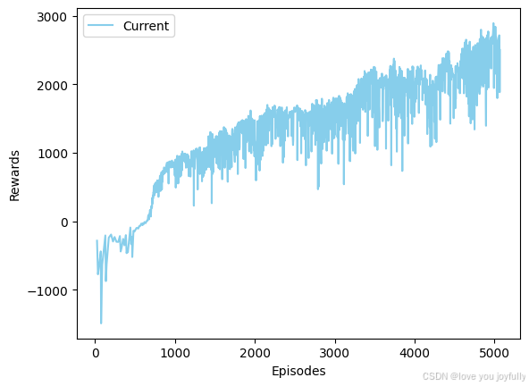

可以看到，训练回报在不断上升，经过一段时间的训练，让我们在Ant环境中看看训练效果吧！

python 复制代码

import matplotlib.pyplot as plt
%matplotlib inline
from IPython import display
import time

def show_state(env, step=0, info=""):
    plt.figure(3)
    plt.clf()
    plt.imshow(env.render())
    plt.axis('off')
    display.clear_output(wait=True)
    display.display(plt.gcf())

env = gym.make('Ant-v4', render_mode='rgb_array')
state, info = env.reset()
for _ in range(200):
    action = ppo.actor_net.choose_action(torch.from_numpy(np.array(state).astype(np.float32)).unsqueeze(0).to(device))[0]
    state, reward, terminated, truncated, info = env.step(action)
    done = truncated or terminated
    show_state(env, action, info)
    time.sleep(0.05)

    if done:
        state, info = env.reset()
env.close()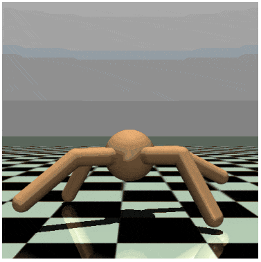

可以看到，此时蚂蚁收敛到了一个"保持不动"的状态，这可能是因为在训练过程中，我们并没有对蚂蚁行走部分施加更加精细有效的奖励，因此蚂蚁只能通过保持不动来获得"局部"最大的回报；或者是训练时间不够长导致的（上述程序在单GPU上运行约需要200~250min）。读者可以设置更加有效的奖励函数，或者增加训练时间，让蚂蚁学会行走。

:::