基于Python+逻辑回归+XGBoost的肝癌预测项目，保存预测模型，基于streamlit快速搭建Web界面，输入患者特征并获取预测结果

一、前期准备：环境配置与数据加载

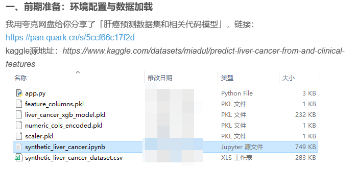
我用夸克网盘给你分享了「肝癌预测数据集和相关代码模型」，链接：https://pan.quark.cn/s/5ccf66c17f2d

kaggle源地址：https://www.kaggle.com/datasets/miadul/predict-liver-cancer-from-and-clinical-features

1. 依赖库

• pandas/numpy：数据读取、清洗与数值计算；
• matplotlib/seaborn：数据可视化；
• scikit-learn：经典机器学习模型（逻辑回归、随机森林等）与评估工具；
• xgboost：高效的梯度提升树模型（适合医疗数据分类）；
• shap：模型可解释性分析（医疗场景需明确"哪些特征导致癌症预测"）。

没有安装上述依赖库可以安装一下，例如：

pip install shap

2. 加载数据并初步探查

通过pandas读取CSV文件，查看数据基本信息（维度、缺失值、数据类型），避免后续因数据格式问题报错：

import pandas as pd
import numpy as np

# 加载数据（需替换为你的数据集本地路径）
df = pd.read_csv("predict_liver_cancer.csv")

# 1. 查看数据前5行，了解特征分布
print("数据前5行：")
print(df.head())

# 2. 查看数据维度（行数×列数）
print(f"\n数据维度：{df.shape}")  # 预期输出 (5000, 14)

# 3. 检查缺失值（该数据集为合成数据，通常无缺失，但需验证）
print("\n各列缺失值数量：")
print(df.isnull().sum())

# 4. 查看数据类型与统计描述
print("\n数据类型：")
print(df.dtypes)
print("\n数值型特征统计描述：")
print(df.describe())  # 仅显示age、bmi等数值列的均值、标准差、分位数等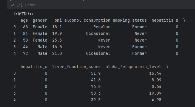

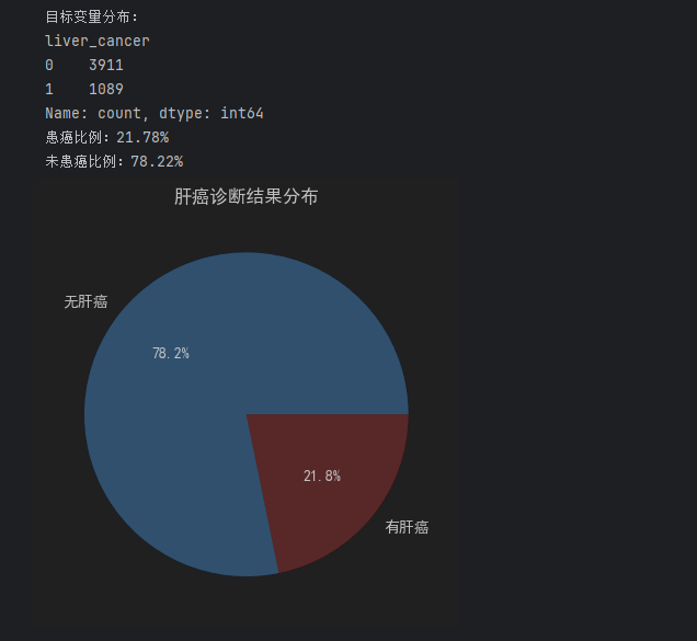
3. 目标变量分布检查

该任务为二分类问题 （预测是否患肝癌：liver_cancer=1/0），需先确认正负样本是否平衡（避免模型偏向多数类）：

# 统计目标变量数量与占比
target_count = df["liver_cancer"].value_counts()
print("目标变量分布：")
print(target_count)
print(f"患癌比例：{target_count[1]/len(df):.2%}")
print(f"未患癌比例：{target_count[0]/len(df):.2%}")

# 可视化目标变量分布（用饼图更直观）
import matplotlib.pyplot as plt
plt.pie(target_count, labels=["无肝癌", "有肝癌"], autopct="%1.1f%%", colors=["#66b3ff", "#ff9999"])
plt.title("肝癌诊断结果分布")
plt.show()

• 如果两类样本比例差异过大（如患癌样本<10%），后续建模需用SMOTE过采样 或类权重调整 （如class_weight='balanced'）解决 imbalance 问题。
  

二、核心环节1：探索性数据分析（EDA）

EDA是理解数据的关键，需从单特征分布、特征与目标的关联、特征间相关性三个维度展开，挖掘医疗数据中的潜在规律（如"肝炎患者是否更易患肝癌""BMI与肝癌的关系"）。

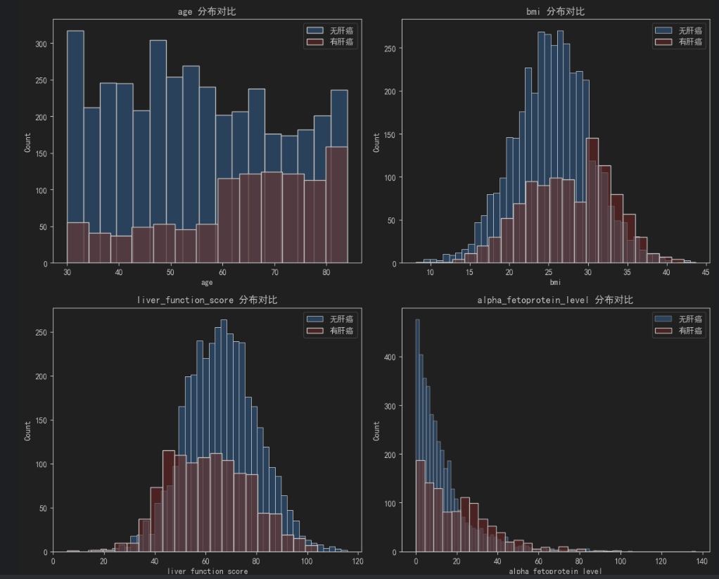
1. 数值型特征分析（年龄、BMI、肝功能评分等）

重点查看数值特征的分布形态，以及不同肝癌诊断结果下的特征差异：

import seaborn as sns

# 定义数值型特征列表（从数据集描述中提取）
numeric_features = ["age", "bmi", "liver_function_score", "alpha_fetoprotein_level"]

# 1. 绘制数值特征的直方图（按肝癌诊断分组，对比分布差异）
fig, axes = plt.subplots(2, 2, figsize=(12, 10))
axes = axes.flatten()  # 展平子图数组，便于循环

for i, feat in enumerate(numeric_features):
    # 无肝癌组
    sns.histplot(df[df["liver_cancer"]==0][feat], ax=axes[i], label="无肝癌", color="#66b3ff", alpha=0.7)
    # 有肝癌组
    sns.histplot(df[df["liver_cancer"]==1][feat], ax=axes[i], label="有肝癌", color="#ff9999", alpha=0.7)
    axes[i].set_title(f"{feat} 分布对比")
    axes[i].legend()

plt.tight_layout()
plt.show()

# 2. 统计不同肝癌状态下数值特征的均值（医疗场景中"均值差异"有临床意义）
numeric_stats = df.groupby("liver_cancer")[numeric_features].mean()
print("不同肝癌状态下数值特征的均值：")
print(numeric_stats)

• 关键观察点：例如alpha_fetoprotein_level（甲胎蛋白，临床肝癌标志物）在"有肝癌"组的均值应显著高于"无肝癌"组，若符合则数据逻辑合理。
  

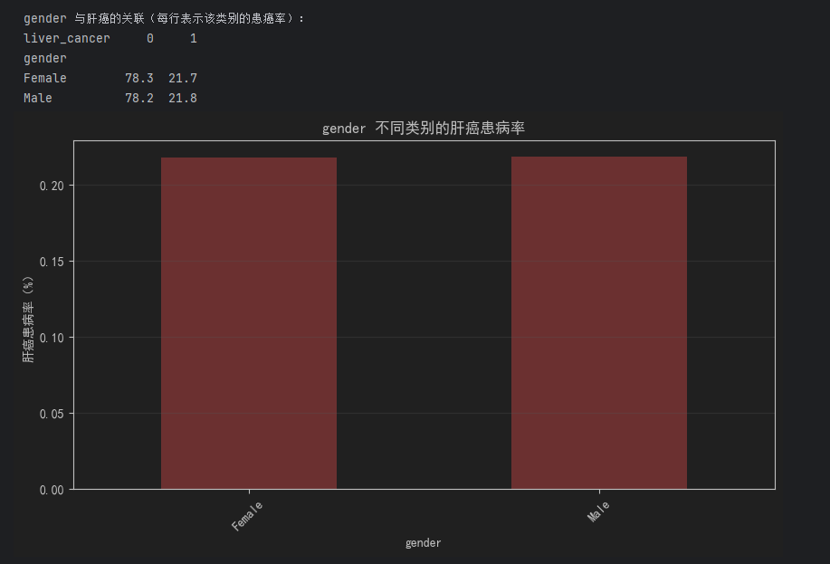
2. 分类型特征分析（性别、饮酒、吸烟、肝炎史等）

分类型特征需用交叉表 或条形图分析其与肝癌的关联（如"男性vs女性的患癌率""有乙肝vs无乙肝的患癌率"）：

# 定义分类型特征列表（含二分类特征如hepatitis_b，及多分类如alcohol_consumption）
cat_features = ["gender", "alcohol_consumption", "smoking_status", "hepatitis_b", "hepatitis_c", "cirrhosis_history", "family_history_cancer", "physical_activity_level", "diabetes"]

# 循环分析每个分类型特征与肝癌的关联
for feat in cat_features:
    # 1. 计算交叉表：特征类别 × 肝癌状态，得到数量分布
    cross_tab = pd.crosstab(df[feat], df["liver_cancer"], normalize="index")  # normalize="index" 计算每行占比（即该类别的患癌率）
    print(f"\n{feat} 与肝癌的关联（每行表示该类别的患癌率）：")
    print(cross_tab.round(3) * 100)  # 转为百分比，保留1位小数
    
    # 2. 可视化：条形图展示不同类别的患癌率
    plt.figure(figsize=(10, 5))
    cross_tab[1].plot(kind="bar", color="#ff6b6b")  # 只展示"患癌率"（liver_cancer=1的列）
    plt.title(f"{feat} 不同类别的肝癌患病率")
    plt.xlabel(feat)
    plt.ylabel("肝癌患病率（%）")
    plt.xticks(rotation=45)
    plt.grid(axis="y", alpha=0.3)
    plt.show()

• 关键医疗逻辑验证：例如cirrhosis_history（肝硬化史）、hepatitis_b（乙肝）组的患癌率应显著高于无病史组，若符合则数据符合医学常识。
  

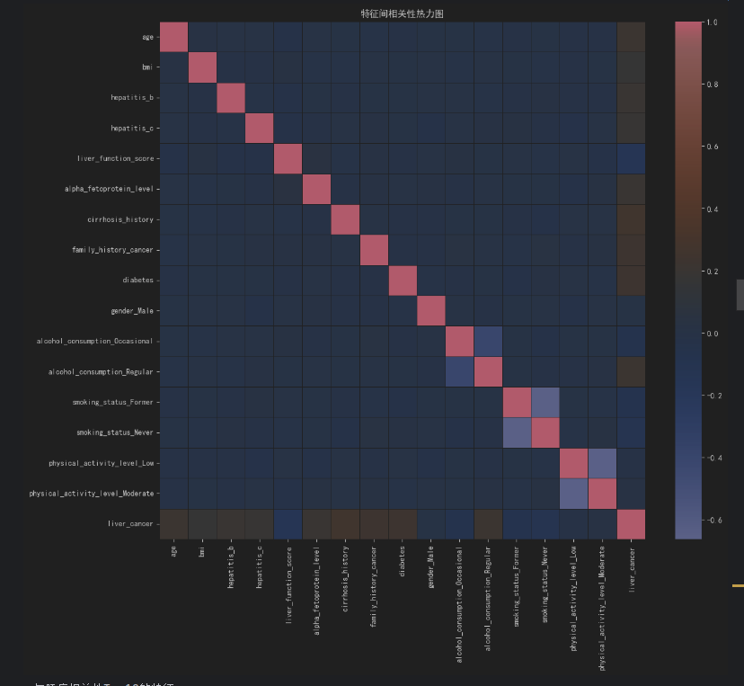
3. 特征间相关性分析

通过热力图查看特征间的线性相关程度，避免建模时的"多重共线性"问题（如两个高度相关的特征可能导致模型系数不稳定）：

# 先将分类型特征转为数值型（one-hot编码），再计算相关系数
df_encoded = pd.get_dummies(df.drop("liver_cancer", axis=1), drop_first=True)  # drop_first避免虚拟变量陷阱
df_encoded["liver_cancer"] = df["liver_cancer"]  # 加回目标变量

# 计算Pearson相关系数
corr_matrix = df_encoded.corr()

# 可视化热力图（重点关注与目标变量的相关性）
plt.figure(figsize=(14, 12))
sns.heatmap(corr_matrix, annot=False, cmap="coolwarm", fmt=".2f", linewidths=0.5)
plt.title("特征间相关性热力图")
plt.show()

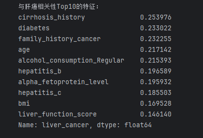
# 提取与"肝癌"相关性Top10的特征（按绝对值排序）
target_corr = corr_matrix["liver_cancer"].drop("liver_cancer").abs().sort_values(ascending=False)
print("与肝癌相关性Top10的特征：")
print(target_corr.head(10))

• 预期结果：alpha_fetoprotein_level（甲胎蛋白）、cirrhosis_history（肝硬化史）、hepatitis_b/c（肝炎）应与目标变量相关性最高，符合临床认知。

三、核心环节2：数据预处理

医疗数据需处理分类型特征编码、数值型特征标准化、样本平衡，确保模型输入格式正确且训练稳定。

from sklearn.model_selection import train_test_split
from sklearn.preprocessing import StandardScaler
from imblearn.over_sampling import SMOTE  # 处理样本不平衡

# 1. 分离特征（X）和目标变量（y）
X = df.drop("liver_cancer", axis=1)
y = df["liver_cancer"]

# 2. 分类型特征编码（one-hot编码，适用于无顺序的类别如gender、alcohol_consumption）
X_encoded = pd.get_dummies(X, drop_first=True)  # drop_first=True：避免多重共线性（如Male=1则Female=0，无需保留Female列）

# 3. 划分训练集和测试集（8:2分割，保证数据分布一致）
X_train, X_test, y_train, y_test = train_test_split(
    X_encoded, y, test_size=0.2, random_state=42, stratify=y  # stratify=y：按目标变量分布分层，保证训练/测试集患癌率一致
)

# 4. 数值型特征标准化（对逻辑回归、SVM等敏感模型必要，消除量纲影响）
# 先筛选数值型特征列（从原始X中提取）
numeric_cols = ["age", "bmi", "liver_function_score", "alpha_fetoprotein_level"]
# 对应到编码后的X_train/X_test的列名（如无变化，直接用原列名）
numeric_cols_encoded = [col for col in numeric_cols if col in X_train.columns]

# 初始化标准化器，仅对数值列标准化
scaler = StandardScaler()
X_train[numeric_cols_encoded] = scaler.fit_transform(X_train[numeric_cols_encoded])
X_test[numeric_cols_encoded] = scaler.transform(X_test[numeric_cols_encoded])  # 测试集用训练集的均值/标准差，避免数据泄露

# 5. 处理样本不平衡（若之前发现患癌样本占比<15%，用SMOTE过采样）
print(f"过采样前训练集患癌样本占比：{y_train.sum()/len(y_train):.2%}")
smote = SMOTE(random_state=42)
X_train_resampled, y_train_resampled = smote.fit_resample(X_train, y_train)
print(f"过采样后训练集患癌样本占比：{y_train_resampled.sum()/len(y_train_resampled):.2%}")  # 预期为50%

四、核心环节3：机器学习建模与评估

医疗场景中，模型的召回率（Recall，避免漏诊）、精确率（Precision，避免误诊）、AUC（整体区分能力） 是关键指标。推荐从"简单基准模型"到"复杂模型"逐步迭代，对比效果。

1. 模型选择与训练

推荐4类适合医疗二分类的模型，覆盖不同复杂度：

模型类型	特点	适用场景
逻辑回归	简单可解释，能输出概率	基线模型，快速验证数据有效性
随机森林	抗过拟合，对异常值鲁棒	处理非线性关系，特征重要性易获取
XGBoost	梯度提升，精度高，适合小样本医疗数据	追求高预测精度
支持向量机（SVM）	高维数据表现好	特征维度高、样本量适中的场景

以下是核心代码（以逻辑回归和XGBoost为例）：

from sklearn.linear_model import LogisticRegression
from xgboost import XGBClassifier
from sklearn.metrics import (
    accuracy_score, precision_score, recall_score, f1_score, roc_auc_score,
    confusion_matrix, classification_report, roc_curve
)

# ---------------------- 1. 基准模型：逻辑回归 ----------------------
lr_model = LogisticRegression(class_weight="balanced", max_iter=1000, random_state=42)
lr_model.fit(X_train_resampled, y_train_resampled)

# 预测（输出概率，便于后续计算AUC）
y_pred_lr = lr_model.predict(X_test)
y_pred_proba_lr = lr_model.predict_proba(X_test)[:, 1]  # 患癌的概率

# ---------------------- 2. 高精度模型：XGBoost ----------------------
xgb_model = XGBClassifier(
    objective="binary:logistic",  # 二分类任务
    eval_metric="auc",            # 评估指标用AUC
    random_state=42,
    learning_rate=0.1,
    n_estimators=100
)
xgb_model.fit(
    X_train_resampled, y_train_resampled,
    eval_set=[(X_test, y_test)],  # 验证集
    early_stopping_rounds=10,     # 早停：10轮无提升则停止，避免过拟合
    verbose=False
)

# 预测
y_pred_xgb = xgb_model.predict(X_test)
y_pred_proba_xgb = xgb_model.predict_proba(X_test)[:, 1]

2. 模型评估（医疗场景重点关注漏诊/误诊）

用混淆矩阵、分类报告、ROC曲线 全面评估模型，尤其关注recall（漏诊率=1-recall，越低越好）和precision（误诊率=1-precision，越低越好）：

# 定义评估函数，简化代码
def evaluate_model(y_true, y_pred, y_pred_proba, model_name):
    print(f"=== {model_name} 评估结果 ===")
    # 混淆矩阵（TP:真阳性，TN:真阴性，FP:假阳性，FN:假阴性）
    cm = confusion_matrix(y_true, y_pred)
    print("混淆矩阵：")
    print(cm)
    # 关键指标
    print(f"准确率（Accuracy）：{accuracy_score(y_true, y_pred):.4f}")
    print(f"精确率（Precision）：{precision_score(y_true, y_pred):.4f}")  # 预测为患癌的人中，实际患癌的比例（避免误诊）
    print(f"召回率（Recall）：{recall_score(y_true, y_pred):.4f}")        # 实际患癌的人中，被正确预测的比例（避免漏诊）
    print(f"F1分数：{f1_score(y_true, y_pred):.4f}")                    # 精确率和召回率的调和平均
    print(f"AUC值：{roc_auc_score(y_true, y_pred_proba):.4f}")          # 整体区分能力（0.9以上为优秀）
    # 分类报告（含每个类别的指标）
    print("分类报告：")
    print(classification_report(y_true, y_pred))
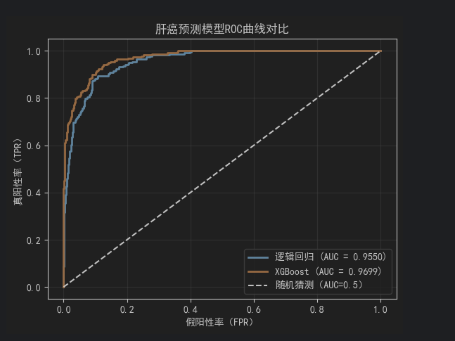
    # 绘制ROC曲线
    fpr, tpr, _ = roc_curve(y_true, y_pred_proba)
    plt.plot(fpr, tpr, label=f"{model_name} (AUC = {roc_auc_score(y_true, y_pred_proba):.4f})", linewidth=2)

# 评估两个模型
evaluate_model(y_test, y_pred_lr, y_pred_proba_lr, "逻辑回归")
evaluate_model(y_test, y_pred_xgb, y_pred_proba_xgb, "XGBoost")

# 绘制ROC曲线对比
plt.plot([0, 1], [0, 1], "k--", label="随机猜测（AUC=0.5）")
plt.xlabel("假阳性率（FPR）")
plt.ylabel("真阳性率（TPR）")
plt.title("肝癌预测模型ROC曲线对比")
plt.legend()
plt.grid(alpha=0.3)
plt.show()

• 医疗场景优先级：若为"早期筛查"，需优先保证高召回率（避免漏诊潜在患者）；若为"确诊辅助"，需平衡召回率和精确率（避免过度医疗）。

五、核心环节4：特征重要性与模型可解释性

医疗AI模型需"可解释"（医生需知道"为什么该患者被预测为患癌"），推荐用逻辑回归系数、随机森林/XGBoost特征重要性、SHAP值三种方式解读：

1. 逻辑回归系数（线性关系解读）

逻辑回归的系数正负表示"特征对患癌的影响方向"，绝对值表示影响强度：

# 提取逻辑回归系数，与特征名对应
lr_coef = pd.DataFrame({
    "feature": X_train.columns,
    "coefficient": lr_model.coef_[0]  # 逻辑回归为二分类，系数数组长度=特征数
})

# 按系数绝对值排序，查看影响最大的特征
lr_coef["abs_coef"] = lr_coef["coefficient"].abs()
lr_coef_sorted = lr_coef.sort_values("abs_coef", ascending=False)

print("逻辑回归：影响肝癌的Top10特征（按系数绝对值）：")
print(lr_coef_sorted.head(10)[["feature", "coefficient"]])

# 可视化Top10特征的系数（正负表示影响方向）
plt.figure(figsize=(12, 6))
sns.barplot(x="coefficient", y="feature", data=lr_coef_sorted.head(10))
plt.title("逻辑回归：影响肝癌的Top10特征（系数）")
plt.xlabel("系数值（正=增加患癌风险，负=降低患癌风险）")
plt.ylabel("特征")
plt.grid(axis="x", alpha=0.3)
plt.show()

• 预期结论：cirrhosis_history_1（有肝硬化史）、hepatitis_b_1（有乙肝）的系数为正且绝对值大，说明这些特征会显著增加患癌风险。

2. XGBoost特征重要性（非线性关系解读）

XGBoost通过"特征在决策树中被使用的次数/增益"衡量重要性，适合解读非线性影响：

# 提取XGBoost特征重要性（两种指标：weight=使用次数，gain=信息增益）
xgb_importance = pd.DataFrame({
    "feature": X_train.columns,
    "weight": xgb_model.feature_importances_  # 默认是weight指标
})

# 按重要性排序
xgb_importance_sorted = xgb_importance.sort_values("weight", ascending=False)

print("XGBoost：影响肝癌的Top10特征（按使用次数）：")
print(xgb_importance_sorted.head(10))

# 可视化Top10特征重要性
plt.figure(figsize=(12, 6))
sns.barplot(x="weight", y="feature", data=xgb_importance_sorted.head(10))
plt.title("XGBoost：影响肝癌的Top10特征（重要性）")
plt.xlabel("特征重要性（weight指标）")
plt.ylabel("特征")
plt.grid(axis="x", alpha=0.3)
plt.show()

3. SHAP值（个体样本解读）

SHAP值可量化"每个特征对单个患者预测结果的贡献"，医生可通过它解释"该患者患癌预测的依据"：

import shap

# 初始化SHAP解释器（XGBoost专用）
explainer = shap.TreeExplainer(xgb_model)
# 计算测试集的SHAP值
shap_values = explainer.shap_values(X_test)

# 1. 总结图：全局特征影响（每个点代表一个样本的SHAP值，颜色代表特征值大小）
plt.figure(figsize=(12, 8))
shap.summary_plot(shap_values, X_test, feature_names=X_train.columns, plot_type="bar")
plt.title("SHAP值：全局特征重要性（Top15）")
plt.show()

# 2. 个体解释图：以测试集中第1个样本为例，解读其预测依据
sample_idx = 0  # 选择第1个测试样本
plt.figure(figsize=(10, 6))
shap.force_plot(
    explainer.expected_value,  # 模型对所有样本的平均预测概率
    shap_values[sample_idx],   # 该样本的SHAP值
    X_test.iloc[sample_idx],   # 该样本的特征值
    feature_names=X_train.columns,
    matplotlib=True
)
plt.title(f"样本{sample_idx}的肝癌预测SHAP解释（红色=增加患癌风险，蓝色=降低风险）")
plt.show()

• 解读逻辑：红色特征块表示"该特征值增加了该患者的患癌概率"（如alpha_fetoprotein_level=80ng/mL，高于均值），蓝色块表示"降低风险"（如hepatitis_b=0，无乙肝）。

六、进阶操作：模型优化与部署

若需进一步提升模型性能或落地应用，可尝试以下方向：

1. 模型超参数优化

用GridSearchCV或RandomizedSearchCV调优参数（以XGBoost为例）：

import pandas as pd
import numpy as np
from sklearn.model_selection import RandomizedSearchCV
from xgboost import XGBClassifier
from imblearn.over_sampling import SMOTE

# 假设X_train、X_test、y_train、y_test已完成前期预处理（编码、标准化）
# 1. 处理数据类型和缺失值
X_train = X_train.astype('float64').fillna(0)
X_test = X_test.astype('float64').fillna(0)

# 2. 重新过采样，确保X和y样本数匹配
smote = SMOTE(random_state=42)
X_train_resampled, y_train_resampled = smote.fit_resample(X_train, y_train)

# 3. 定义XGBoost基础模型（不含搜索参数）
xgb_model = XGBClassifier(
    objective="binary:logistic",
    eval_metric="auc",
    random_state=42
)

# 4. 定义参数搜索空间
param_grid = {
    "learning_rate": [0.01, 0.1, 0.2],
    "n_estimators": [50, 100, 200],
    "max_depth": [3, 5, 7],
    "subsample": [0.8, 1.0],
    "colsample_bytree": [0.8, 1.0]
}

# 5. 随机搜索
random_search = RandomizedSearchCV(
    estimator=xgb_model,
    param_distributions=param_grid,
    n_iter=20,
    cv=5,
    scoring="roc_auc",
    random_state=42,
    verbose=1
)

# 6. 训练（此时应无报错）
random_search.fit(X_train_resampled, y_train_resampled)

# 后续操作...
print("XGBoost最优参数：", random_search.best_params_)
best_xgb_model = random_search.best_estimator_
y_pred_best_xgb = best_xgb_model.predict(X_test)

2. 模型部署（简易Web应用）

用Streamlit快速搭建Web界面，供医生输入患者特征并获取预测结果：

# 安装Streamlit：pip install streamlit
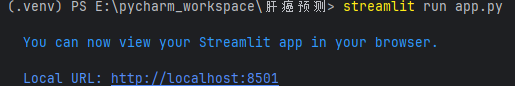
# 保存为app.py，运行：streamlit run app.py

import streamlit as st
import pandas as pd

# 加载训练好的模型和标准化器（需提前用joblib保存）
import joblib
joblib.dump(best_xgb_model, "liver_cancer_xgb_model.pkl")
joblib.dump(scaler, "scaler.pkl")
joblib.dump(X_train.columns, "feature_columns.pkl")

# 加载模型
model = joblib.load("liver_cancer_xgb_model.pkl")
scaler = joblib.load("scaler.pkl")
feature_cols = joblib.load("feature_columns.pkl")

# Web界面设计
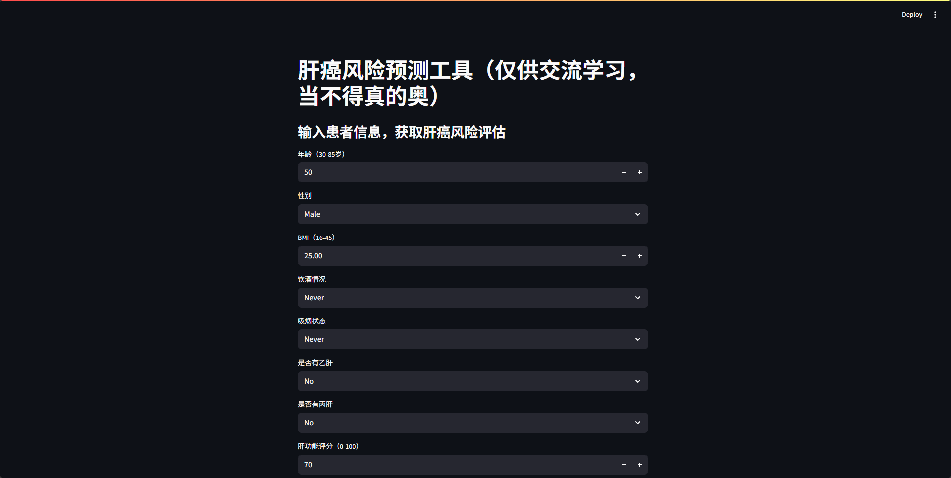
st.title("肝癌风险预测工具")
st.subheader("输入患者信息，获取肝癌风险评估")

# 1. 收集用户输入（对应数据集的13个特征）
age = st.number_input("年龄（30-85岁）", min_value=30, max_value=85, value=50)
gender = st.selectbox("性别", ["Male", "Female"])
bmi = st.number_input("BMI（16-45）", min_value=16.0, max_value=45.0, value=25.0)
alcohol = st.selectbox("饮酒情况", ["Never", "Occasional", "Regular"])
smoking = st.selectbox("吸烟状态", ["Never", "Former", "Current"])
hepatitis_b = st.selectbox("是否有乙肝", ["No", "Yes"])
hepatitis_c = st.selectbox("是否有丙肝", ["No", "Yes"])
liver_score = st.number_input("肝功能评分（0-100）", min_value=0, max_value=100, value=70)
afp = st.number_input("甲胎蛋白水平（ng/mL）", min_value=0.0, value=10.0)
cirrhosis = st.selectbox("是否有肝硬化史", ["No", "Yes"])
family_cancer = st.selectbox("是否有癌症家族史", ["No", "Yes"])
activity = st.selectbox("体力活动水平", ["Low", "Moderate", "High"])
diabetes = st.selectbox("是否有糖尿病", ["No", "Yes"])

# 2. 将输入转为DataFrame，与训练数据格式一致
input_data = pd.DataFrame({
    "age": [age],
    "gender": [gender],
    "bmi": [bmi],
    "alcohol_consumption": [alcohol],
    "smoking_status": [smoking],
    "hepatitis_b": [1 if hepatitis_b=="Yes" else 0],
    "hepatitis_c": [1 if hepatitis_c=="Yes" else 0],
    "liver_function_score": [liver_score],
    "alpha_fetoprotein_level": [afp],
    "cirrhosis_history": [1 if cirrhosis=="Yes" else 0],
    "family_history_cancer": [1 if family_cancer=="Yes" else 0],
    "physical_activity_level": [activity],
    "diabetes": [1 if diabetes=="Yes" else 0]
})

# 3. 预处理输入数据（与训练流程一致）
input_encoded = pd.get_dummies(input_data, drop_first=True)
# 确保输入特征与训练集完全一致（补充缺失的虚拟变量列，值为0）
for col in feature_cols:
    if col not in input_encoded.columns:
        input_encoded[col] = 0
input_encoded = input_encoded[feature_cols]  # 调整列顺序

# 4. 标准化数值特征
input_encoded[numeric_cols_encoded] = scaler.transform(input_encoded[numeric_cols_encoded])

# 5. 预测并展示结果
if st.button("预测肝癌风险"):
    prob = model.predict_proba(input_encoded)[0, 1]  # 患癌概率
    st.subheader(f"预测结果：")
    if prob >= 0.5:
        st.warning(f"该患者患肝癌的概率为 {prob:.2%}，建议进一步临床检查！")
    else:
        st.success(f"该患者患肝癌的概率为 {prob:.2%}，风险较低。")

七、总结与注意事项

1. 数据特性适配：该数据集为合成数据，无真实患者隐私问题，可放心用于实验，但实际医疗场景需严格遵守HIPAA、隐私保护法等规范。
2. 医疗逻辑优先：建模过程中需结合医学常识（如甲胎蛋白、肝炎史是肝癌关键风险因素），若特征重要性与临床认知冲突，需检查数据或模型问题。
3. 模型局限性：机器学习模型仅为"辅助工具"，不能替代医生诊断，需在结果中明确标注"预测结果仅供参考，以临床检查为准"。

八、如何运行streamlit快速搭建Web界面

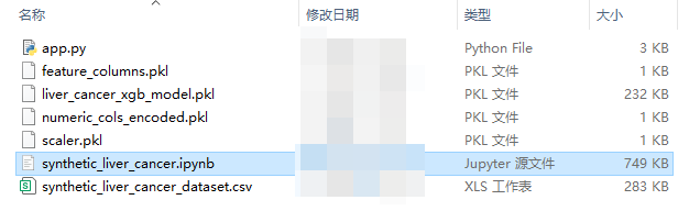
1、下载运行文件和模型文件

先把下面的这个文件下载下来，这是在标题一里呢。

2、进入你存放项目文件的文件夹

点击右侧控制台，cd到你存放文件的地方

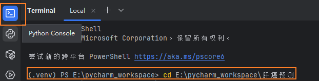
3、输入以下命令运行

streamlit run app.py