[机器学习]基于K-means聚类算法的鸢尾花数据及分类

基于Kmeans，对鸢尾花数据集前两个特征进行聚类分析

通过迭代优化，将150个样本划分到K个簇中。
目标函数：最小化所有样本到其所属簇中心的距离平方和。
算法步骤：
1. 随机初始化K个簇中心。
2. 将每个样本分配到最近的中心。
3. 计算均值确定每个簇的中心（均值）。
4. 重复第2和3步直到稳定收敛。

程序代码：

python 复制代码

import math

import numpy as np
from matplotlib import pyplot as plt
from sklearn import datasets

plt.rcParams['font.sans-serif'] = ['SimHei']
plt.rcParams['axes.unicode_minus'] = False

data = datasets.load_iris().data
labels = datasets.load_iris().target
print('数据维度',data.shape)
features = data[:,: 2]
print('特征',features)

num_clusters = 6
epoch = 150
J_sum = []

def J_calculate(features,divide_re,center):
    J = 0
    for s1 in range(150):
        distances = ((features[s1][0]-center[divide_re[s1]][0]) ** 2) + ((features[s1][1]-center[divide_re[s1]][1]) ** 2)
        #print(distances)
        J = J + distances
    return J

def decision(features,divide_re,center,epoch):
    J_best = []
    for _ in range(epoch):
        J_b = math.inf
        for s1 in range(150):
            best = None
            min_J_now = math.inf
            for s2 in range(len(center)):
                divide_re[s1] = s2
                J_now = J_calculate(features,divide_re,center)
                if J_now < min_J_now:
                    min_J_now = J_now
                    best = s2
            divide_re[s1] = best
            for i in range(len(center)):
                xc = []
                yc = []
                for j in range(150):
                    if (divide_re[j] == i):
                        xc.append(features[j][0])
                        yc.append(features[j][1])
                center[i] = [np.mean(xc), np.mean(yc)]

            if(min_J_now<J_b):
                J_b = min_J_now
        J_best.append(J_b)

    return features,divide_re,center,J_best

for i in range(2,num_clusters+1):
    print(f'\n分{i}类:\n')
    center = features[np.random.choice(features.shape[0], i, replace=False)]
    print("初始中心点", center)
    distances = np.linalg.norm(features[:, np.newaxis, :] - center, axis=2)
    divide = np.argmin(distances,axis=1)
    divide_re = []
    for x in range(150):
        divide_re.append(divide[x])
    print("初始样本分类", divide_re)
    features,divide_re,center,J_best = decision(features,divide_re,center,epoch)
    print(f'{i}类最佳J值为:',J_best[epoch-1])
    J_sum.append(J_best[epoch-1])
    plt.scatter(features[:, 0], features[:, 1], c=divide_re, cmap='viridis', edgecolors='k')
    plt.scatter(center[:, 0], center[:, 1], marker='x', s=30, linewidths=3, color='red')
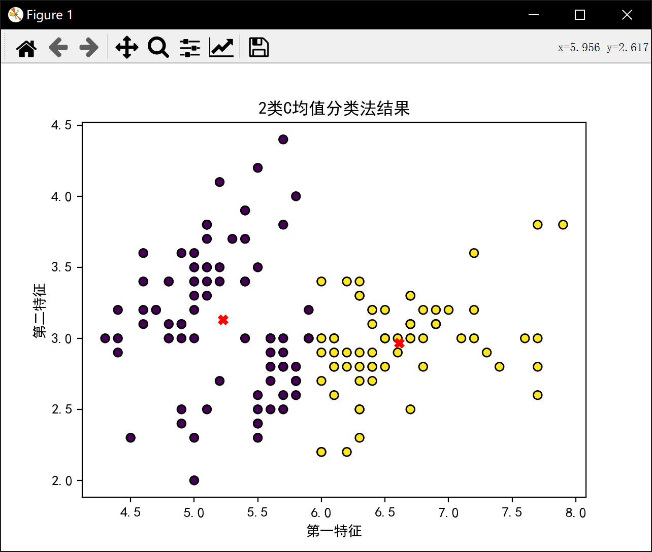
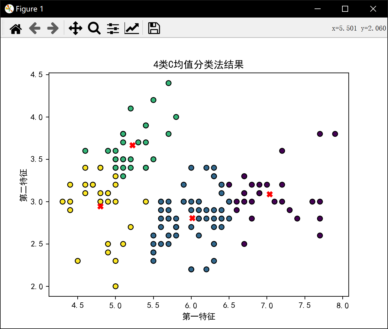
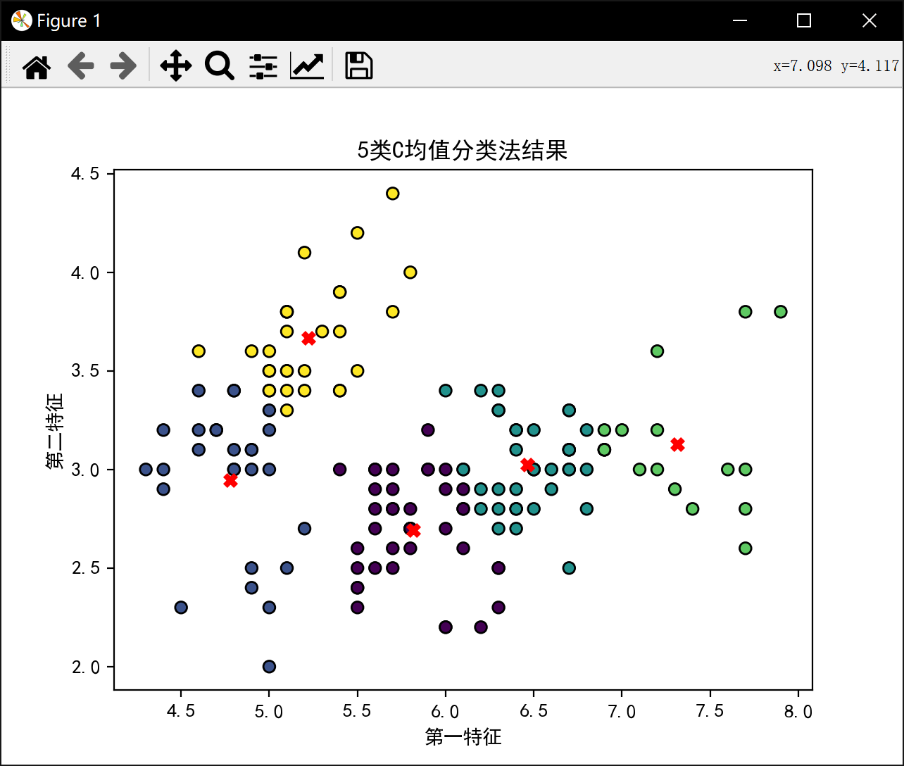
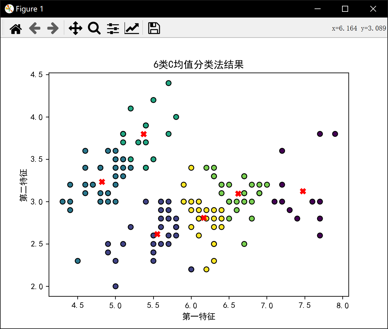
    plt.title(f'{i}类C均值分类法结果')
    plt.xlabel('第一特征')
    plt.ylabel('第二特征')
    plt.show()
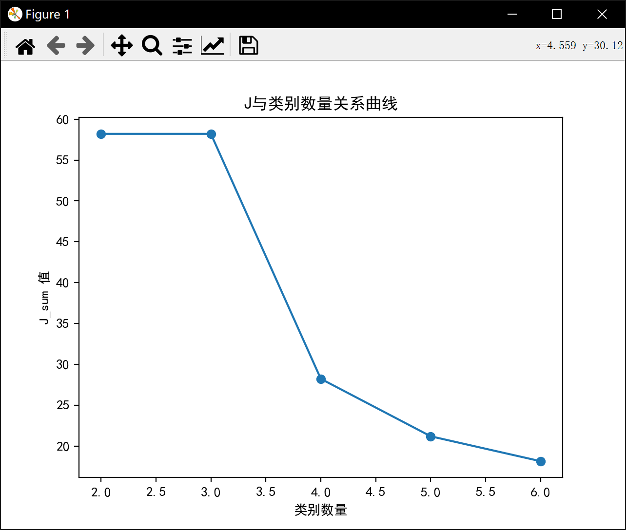
plt.figure()
plt.plot(range(2, num_clusters + 1), J_sum, marker='o')
plt.title('J与类别数量关系曲线')
plt.xlabel('类别数量')
plt.ylabel('J_sum 值')
plt.show()

运行结果：

数据维度 (150, 4)

特征 $\[5.1 3.5$
$4.9 3.$ $4.7 3.2$ $4.6 3.1$ $5. 3.6$ $5.4 3.9$ $4.6 3.4$ $5. 3.4$ $4.4 2.9$ $4.9 3.1$ $5.4 3.7$ $4.8 3.4$ $4.8 3.$ $4.3 3.$ $5.8 4.$ $5.7 4.4$ $5.4 3.9$ $5.1 3.5$ $5.7 3.8$ $5.1 3.8$ $5.4 3.4$ $5.1 3.7$ $4.6 3.6$ $5.1 3.3$ $4.8 3.4$ $5. 3.$ $5. 3.4$ $5.2 3.5$ $5.2 3.4$ $4.7 3.2$ $4.8 3.1$ $5.4 3.4$ $5.2 4.1$ $5.5 4.2$ $4.9 3.1$ $5. 3.2$ $5.5 3.5$ $4.9 3.6$ $4.4 3.$ $5.1 3.4$ $5. 3.5$ $4.5 2.3$ $4.4 3.2$ $5. 3.5$ $5.1 3.8$ $4.8 3.$ $5.1 3.8$ $4.6 3.2$ $5.3 3.7$ $5. 3.3$ $7. 3.2$ $6.4 3.2$ $6.9 3.1$ $5.5 2.3$ $6.5 2.8$ $5.7 2.8$ $6.3 3.3$ $4.9 2.4$ $6.6 2.9$ $5.2 2.7$ $5. 2.$ $5.9 3.$ $6. 2.2$ $6.1 2.9$ $5.6 2.9$ $6.7 3.1$ $5.6 3.$ $5.8 2.7$ $6.2 2.2$ $5.6 2.5$ $5.9 3.2$ $6.1 2.8$ $6.3 2.5$ $6.1 2.8$ $6.4 2.9$ $6.6 3.$ $6.8 2.8$ $6.7 3.$ $6. 2.9$ $5.7 2.6$ $5.5 2.4$ $5.5 2.4$ $5.8 2.7$ $6. 2.7$ $5.4 3.$ $6. 3.4$ $6.7 3.1$ $6.3 2.3$ $5.6 3.$ $5.5 2.5$ $5.5 2.6$ $6.1 3.$ $5.8 2.6$ $5. 2.3$ $5.6 2.7$ $5.7 3.$ $5.7 2.9$ $6.2 2.9$ $5.1 2.5$ $5.7 2.8$ $6.3 3.3$ $5.8 2.7$ $7.1 3.$ $6.3 2.9$ $6.5 3.$ $7.6 3.$ $4.9 2.5$ $7.3 2.9$ $6.7 2.5$ $7.2 3.6$ $6.5 3.2$ $6.4 2.7$ $6.8 3.$ $5.7 2.5$ $5.8 2.8$ $6.4 3.2$ $6.5 3.$ $7.7 3.8$ $7.7 2.6$ $6. 2.2$ $6.9 3.2$ $5.6 2.8$ $7.7 2.8$ $6.3 2.7$ $6.7 3.3$ $7.2 3.2$ $6.2 2.8$ $6.1 3.$ $6.4 2.8$ $7.2 3.$ $7.4 2.8$ $7.9 3.8$ $6.4 2.8$ $6.3 2.8$ $6.1 2.6$ $7.7 3.$ $6.3 3.4$ $6.4 3.1$ $6. 3.$ $6.9 3.1$ $6.7 3.1$ $6.9 3.1$ $5.8 2.7$ $6.8 3.2$ $6.7 3.3$ $6.7 3.$ $6.3 2.5$ $6.5 3.$ $6.2 3.4$ $5.9 3. \]$
分2类:

初始中心点 $\[6.4 3.1$
$7.2 3.6\]$
初始样本分类 $0, 0, 0, 0, 0, 0, 0, 0, 0, 0, 0, 0, 0, 0, 0, 0, 0, 0, 0, 0, 0, 0, 0, 0, 0, 0, 0, 0, 0, 0, 0, 0, 0, 0, 0, 0, 0, 0, 0, 0, 0, 0, 0, 0, 0, 0, 0, 0, 0, 0, 1, 0, 0, 0, 0, 0, 0, 0, 0, 0, 0, 0, 0, 0, 0, 0, 0, 0, 0, 0, 0, 0, 0, 0, 0, 0, 0, 0, 0, 0, 0, 0, 0, 0, 0, 0, 0, 0, 0, 0, 0, 0, 0, 0, 0, 0, 0, 0, 0, 0, 0, 0, 1, 0, 0, 1, 0, 1, 0, 1, 0, 0, 0, 0, 0, 0, 0, 1, 1, 0, 1, 0, 1, 0, 0, 1, 0, 0, 0, 1, 1, 1, 0, 0, 0, 1, 0, 0, 0, 0, 0, 0, 0, 0, 0, 0, 0, 0, 0, 0$

2类最佳J值为: 58.20409278906674

分3类:

初始中心点 $\[5.4 3.4$
$5.4 3.4$ $7.7 2.8\]$
初始样本分类 $0, 0, 0, 0, 0, 0, 0, 0, 0, 0, 0, 0, 0, 0, 0, 0, 0, 0, 0, 0, 0, 0, 0, 0, 0, 0, 0, 0, 0, 0, 0, 0, 0, 0, 0, 0, 0, 0, 0, 0, 0, 0, 0, 0, 0, 0, 0, 0, 0, 0, 2, 0, 2, 0, 2, 0, 0, 0, 2, 0, 0, 0, 0, 0, 0, 2, 0, 0, 0, 0, 0, 0, 0, 0, 0, 2, 2, 2, 0, 0, 0, 0, 0, 0, 0, 0, 2, 0, 0, 0, 0, 0, 0, 0, 0, 0, 0, 0, 0, 0, 0, 0, 2, 0, 0, 2, 0, 2, 2, 2, 0, 0, 2, 0, 0, 0, 0, 2, 2, 0, 2, 0, 2, 0, 2, 2, 0, 0, 0, 2, 2, 2, 0, 0, 0, 2, 0, 0, 0, 2, 2, 2, 0, 2, 2, 2, 0, 0, 0, 0$

3类最佳J值为: 58.20409278906674

分4类:

初始中心点 $\[6.7 3.1$
$6.4 2.7$ $6.5 3.2$ $5.5 2.4\]$
初始样本分类 $3, 3, 3, 3, 3, 2, 3, 3, 3, 3, 2, 3, 3, 3, 2, 2, 2, 3, 2, 3, 3, 3, 3, 3, 3, 3, 3, 3, 3, 3, 3, 3, 2, 2, 3, 3, 2, 3, 3, 3, 3, 3, 3, 3, 3, 3, 3, 3, 2, 3, 0, 2, 0, 3, 1, 3, 2, 3, 0, 3, 3, 1, 3, 1, 3, 0, 3, 3, 1, 3, 2, 1, 1, 1, 1, 0, 0, 0, 1, 3, 3, 3, 3, 1, 3, 2, 0, 1, 3, 3, 3, 1, 3, 3, 3, 3, 3, 1, 3, 3, 2, 3, 0, 1, 2, 0, 3, 0, 1, 0, 2, 1, 0, 3, 3, 2, 2, 0, 0, 3, 0, 3, 0, 1, 0, 0, 1, 1, 1, 0, 0, 0, 1, 1, 1, 0, 2, 2, 1, 0, 0, 0, 3, 0, 0, 0, 1, 2, 2, 1$

4类最佳J值为: 28.23339146670904

分5类:

初始中心点 $\[6.3 2.5$
$5.1 3.5$ $6.4 3.2$ $7.1 3.$ $5.5 3.5\]$
初始样本分类 $1, 1, 1, 1, 1, 4, 1, 1, 1, 1, 4, 1, 1, 1, 4, 4, 4, 1, 4, 1, 4, 1, 1, 1, 1, 1, 1, 1, 1, 1, 1, 4, 1, 4, 1, 1, 4, 1, 1, 1, 1, 1, 1, 1, 1, 1, 1, 1, 1, 1, 3, 2, 3, 0, 0, 0, 2, 1, 2, 1, 0, 2, 0, 2, 4, 2, 4, 0, 0, 0, 2, 0, 0, 0, 2, 2, 3, 2, 0, 0, 0, 0, 0, 0, 4, 2, 2, 0, 4, 0, 0, 2, 0, 1, 0, 4, 4, 2, 1, 0, 2, 0, 3, 2, 2, 3, 1, 3, 0, 3, 2, 0, 3, 0, 0, 2, 2, 3, 3, 0, 3, 4, 3, 0, 2, 3, 0, 2, 0, 3, 3, 3, 0, 0, 0, 3, 2, 2, 2, 3, 2, 3, 0, 3, 2, 2, 0, 2, 2, 2$

5类最佳J值为: 21.200013093214928

分6类:

初始中心点 $\[6.8 2.8$
$5.8 2.6$ $4.4 3.$ $6.2 3.4$ $6.4 3.2$ $6. 3. \]$
初始样本分类 $2, 2, 2, 2, 2, 3, 2, 2, 2, 2, 3, 2, 2, 2, 3, 3, 3, 2, 3, 2, 5, 2, 2, 2, 2, 2, 2, 2, 2, 2, 2, 5, 3, 3, 2, 2, 5, 2, 2, 2, 2, 2, 2, 2, 2, 2, 2, 2, 3, 2, 0, 4, 0, 1, 0, 1, 3, 2, 0, 1, 1, 5, 1, 5, 1, 4, 5, 1, 1, 1, 5, 5, 1, 5, 4, 4, 0, 0, 5, 1, 1, 1, 1, 1, 1, 3, 4, 1, 5, 1, 1, 5, 1, 1, 1, 5, 1, 5, 1, 1, 3, 1, 0, 5, 4, 0, 2, 0, 0, 4, 4, 0, 0, 1, 1, 4, 4, 0, 0, 1, 0, 1, 0, 5, 4, 0, 5, 5, 0, 0, 0, 0, 0, 5, 1, 0, 3, 4, 5, 0, 4, 0, 1, 4, 4, 0, 1, 4, 3, 5$

6类最佳J值为: 18.150987445152886

进程已结束,退出代码0