RLHF-奖励模型RM 的“引擎”：Pairwise Loss 梯度计算详解

RLHF-奖励模型RM 的"引擎"：Pairwise Loss 梯度计算详解

在上一篇文章中，我们介绍了奖励模型 (RM) 是 RLHF 的"指南针"，它通过 Pairwise Ranking Loss 来学习人类的偏好。我们最终得到了一个损失值，例如 0.312。

但这个数字本身并不能更新模型。真正驱动模型学习的，是这个损失值 (Loss) 相对于模型每一个参数 ( <math xmlns="http://www.w3.org/1998/Math/MathML"> θ \theta </math>θ) 的梯度 (Gradient) 。梯度是一个向量，它指明了参数调整的方向，以最快地降低损失。

这篇文章将深入技术细节，拆解 Pairwise Ranking Loss 的反向传播（Backpropagation）过程，揭示模型是如何通过数学"理解"并"执行"------"拉高赢家分数，压低输家分数"这一指令的。

一、 目标与链式法则：拆解依赖关系

我们的总目标是计算 <math xmlns="http://www.w3.org/1998/Math/MathML"> ∇ θ L \nabla_\theta L </math>∇θL，即总损失 <math xmlns="http://www.w3.org/1998/Math/MathML"> L L </math>L 相对于模型所有参数 <math xmlns="http://www.w3.org/1998/Math/MathML"> θ \theta </math>θ 的梯度。

首先，我们回顾一下（为简化起见，我们先忽略平均值 <math xmlns="http://www.w3.org/1998/Math/MathML"> 1 / ( K 2 ) 1/\binom{K}{2} </math>1/(2K)）：
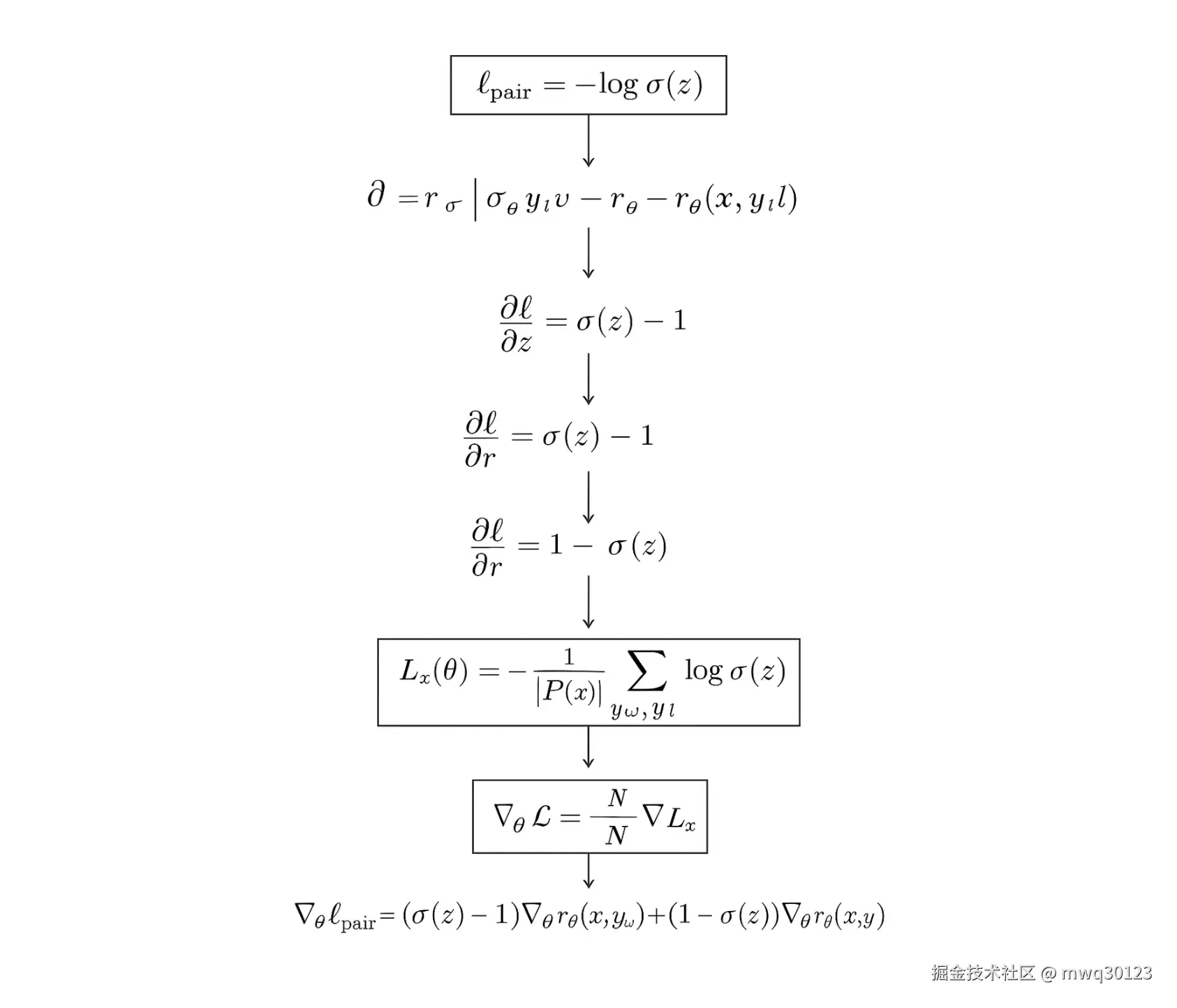
<math xmlns="http://www.w3.org/1998/Math/MathML" display="block"> L ( θ ) = − ∑ ( y w , y l ) log ⁡ ( σ ( r θ ( x , y w ) − r θ ( x , y l ) ) ) L(\theta) = - \sum_{(y_w, y_l)} \log\left(\sigma\left(r_\theta(x, y_w) - r_\theta(x, y_l)\right)\right) </math>L(θ)=−(yw,yl)∑log(σ(rθ(x,yw)−rθ(x,yl)))

我们来看其中一个偏好对 <math xmlns="http://www.w3.org/1998/Math/MathML"> ( y w , y l ) (y_w, y_l) </math>(yw,yl) 产生的损失 <math xmlns="http://www.w3.org/1998/Math/MathML"> L pair L_{\text{pair}} </math>Lpair：
<math xmlns="http://www.w3.org/1998/Math/MathML" display="block"> L pair = − log ⁡ ( σ ( s ) ) 其中 s = r w − r l L_{\text{pair}} = - \log(\sigma(s)) \quad \text{其中 } s = r_w - r_l </math>Lpair=−log(σ(s))其中 s=rw−rl

(注： <math xmlns="http://www.w3.org/1998/Math/MathML"> r w = r θ ( x , y w ) r_w = r_\theta(x, y_w) </math>rw=rθ(x,yw)， <math xmlns="http://www.w3.org/1998/Math/MathML"> r l = r θ ( x , y l ) r_l = r_\theta(x, y_l) </math>rl=rθ(x,yl))

要计算 <math xmlns="http://www.w3.org/1998/Math/MathML"> L pair L_{\text{pair}} </math>Lpair 对 <math xmlns="http://www.w3.org/1998/Math/MathML"> θ \theta </math>θ 的梯度 <math xmlns="http://www.w3.org/1998/Math/MathML"> ∂ L pair ∂ θ \frac{\partial L_{\text{pair}}}{\partial \theta} </math>∂θ∂Lpair，我们必须使用链式法则 (Chain Rule) 。参数 <math xmlns="http://www.w3.org/1998/Math/MathML"> θ \theta </math>θ 的改变是通过影响 <math xmlns="http://www.w3.org/1998/Math/MathML"> r w r_w </math>rw 和 <math xmlns="http://www.w3.org/1998/Math/MathML"> r l r_l </math>rl 的分数，进而影响 <math xmlns="http://www.w3.org/1998/Math/MathML"> s s </math>s 的差值，最后影响 <math xmlns="http://www.w3.org/1998/Math/MathML"> L pair L_{\text{pair}} </math>Lpair 的。

这个过程有两条路径：

1. 路径 1 (通过赢家 <math xmlns="http://www.w3.org/1998/Math/MathML"> r w r_w </math>rw)： <math xmlns="http://www.w3.org/1998/Math/MathML"> θ → r w → s → L pair \theta \to r_w \to s \to L_{\text{pair}} </math>θ→rw→s→Lpair
2. 路径 2 (通过输家 <math xmlns="http://www.w3.org/1998/Math/MathML"> r l r_l </math>rl)： <math xmlns="http://www.w3.org/1998/Math/MathML"> θ → r l → s → L pair \theta \to r_l \to s \to L_{\text{pair}} </math>θ→rl→s→Lpair

因此，总梯度是这两条路径上的梯度之和：
<math xmlns="http://www.w3.org/1998/Math/MathML" display="block"> ∇ θ L pair = ( ∂ L pair ∂ s ⋅ ∂ s ∂ r w ) ⋅ ∇ θ r w + ( ∂ L pair ∂ s ⋅ ∂ s ∂ r l ) ⋅ ∇ θ r l \nabla_\theta L_{\text{pair}} = \left( \frac{\partial L_{\text{pair}}}{\partial s} \cdot \frac{\partial s}{\partial r_w} \right) \cdot \nabla_\theta r_w + \left( \frac{\partial L_{\text{pair}}}{\partial s} \cdot \frac{\partial s}{\partial r_l} \right) \cdot \nabla_\theta r_l </math>∇θLpair=(∂s∂Lpair⋅∂rw∂s)⋅∇θrw+(∂s∂Lpair⋅∂rl∂s)⋅∇θrl

我们可以把这个过程分为两类关键的偏导数进行计算。

二、 第 1 类：损失 L 对分数 r 的偏导数（"上游梯度"）

这是最核心的数学推导，它定义了 Loss 函数本身的行为。

首先，我们使用一个在数值上更稳定的 <math xmlns="http://www.w3.org/1998/Math/MathML"> L pair L_{\text{pair}} </math>Lpair 表达式。

因为 <math xmlns="http://www.w3.org/1998/Math/MathML"> L pair = − log ⁡ ( σ ( s ) ) = − log ⁡ ( 1 1 + e − s ) = log ⁡ ( 1 + e − s ) L_{\text{pair}} = -\log(\sigma(s)) = -\log\left(\frac{1}{1 + e^{-s}}\right) = \log(1 + e^{-s}) </math>Lpair=−log(σ(s))=−log(1+e−s1)=log(1+e−s)。

1. 计算 <math xmlns="http://www.w3.org/1998/Math/MathML"> ∂ L pair ∂ s \frac{\partial L_{\text{pair}}}{\partial s} </math>∂s∂Lpair (损失对分数 差值 的偏导数):

<math xmlns="http://www.w3.org/1998/Math/MathML" display="block"> ∂ L pair ∂ s = d d s log ⁡ ( 1 + e − s ) = 1 1 + e − s ⋅ ( e − s ⋅ − 1 ) \frac{\partial L_{\text{pair}}}{\partial s} = \frac{d}{ds} \log(1 + e^{-s}) = \frac{1}{1 + e^{-s}} \cdot (e^{-s} \cdot -1) </math>∂s∂Lpair=dsdlog(1+e−s)=1+e−s1⋅(e−s⋅−1)
<math xmlns="http://www.w3.org/1998/Math/MathML" display="block"> = − e − s 1 + e − s = − 1 e s + 1 = − σ ( − s ) = σ ( s ) − 1 = - \frac{e^{-s}}{1 + e^{-s}} = - \frac{1}{e^s + 1} = - \sigma(-s) = \sigma(s) - 1 </math>=−1+e−se−s=−es+11=−σ(−s)=σ(s)−1

这个结果 <math xmlns="http://www.w3.org/1998/Math/MathML"> σ ( s ) − 1 \sigma(s) - 1 </math>σ(s)−1 非常关键。

2. 计算 <math xmlns="http://www.w3.org/1998/Math/MathML"> ∂ L pair ∂ r w \frac{\partial L_{\text{pair}}}{\partial r_w} </math>∂rw∂Lpair (损失对 赢家分数 的偏导数):

<math xmlns="http://www.w3.org/1998/Math/MathML" display="block"> ∂ L pair ∂ r w = ∂ L pair ∂ s ⋅ ∂ s ∂ r w \frac{\partial L_{\text{pair}}}{\partial r_w} = \frac{\partial L_{\text{pair}}}{\partial s} \cdot \frac{\partial s}{\partial r_w} </math>∂rw∂Lpair=∂s∂Lpair⋅∂rw∂s

由于 <math xmlns="http://www.w3.org/1998/Math/MathML"> s = r w − r l s = r_w - r_l </math>s=rw−rl，我们知道 <math xmlns="http://www.w3.org/1998/Math/MathML"> ∂ s ∂ r w = 1 \frac{\partial s}{\partial r_w} = 1 </math>∂rw∂s=1。
<math xmlns="http://www.w3.org/1998/Math/MathML" display="block"> ∂ L pair ∂ r w = ( σ ( s ) − 1 ) ⋅ 1 = σ ( r w − r l ) − 1 \frac{\partial L_{\text{pair}}}{\partial r_w} = (\sigma(s) - 1) \cdot 1 = \sigma(r_w - r_l) - 1 </math>∂rw∂Lpair=(σ(s)−1)⋅1=σ(rw−rl)−1

3. 计算 <math xmlns="http://www.w3.org/1998/Math/MathML"> ∂ L pair ∂ r l \frac{\partial L_{\text{pair}}}{\partial r_l} </math>∂rl∂Lpair (损失对 输家分数 的偏导数):

<math xmlns="http://www.w3.org/1998/Math/MathML" display="block"> ∂ L pair ∂ r l = ∂ L pair ∂ s ⋅ ∂ s ∂ r l \frac{\partial L_{\text{pair}}}{\partial r_l} = \frac{\partial L_{\text{pair}}}{\partial s} \cdot \frac{\partial s}{\partial r_l} </math>∂rl∂Lpair=∂s∂Lpair⋅∂rl∂s

由于 <math xmlns="http://www.w3.org/1998/Math/MathML"> s = r w − r l s = r_w - r_l </math>s=rw−rl，我们知道 <math xmlns="http://www.w3.org/1998/Math/MathML"> ∂ s ∂ r l = − 1 \frac{\partial s}{\partial r_l} = -1 </math>∂rl∂s=−1。
<math xmlns="http://www.w3.org/1998/Math/MathML" display="block"> ∂ L pair ∂ r l = ( σ ( s ) − 1 ) ⋅ ( − 1 ) = 1 − σ ( r w − r l ) \frac{\partial L_{\text{pair}}}{\partial r_l} = (\sigma(s) - 1) \cdot (-1) = 1 - \sigma(r_w - r_l) </math>∂rl∂Lpair=(σ(s)−1)⋅(−1)=1−σ(rw−rl)

结果分析：

• 对赢家 <math xmlns="http://www.w3.org/1998/Math/MathML"> r w r_w </math>rw 的梯度 <math xmlns="http://www.w3.org/1998/Math/MathML"> ∂ L pair ∂ r w = σ ( s ) − 1 \frac{\partial L_{\text{pair}}}{\partial r_w} = \sigma(s) - 1 </math>∂rw∂Lpair=σ(s)−1：

  由于 <math xmlns="http://www.w3.org/1998/Math/MathML"> σ ( s ) \sigma(s) </math>σ(s) 的值域在 <math xmlns="http://www.w3.org/1998/Math/MathML"> ( 0 , 1 ) (0, 1) </math>(0,1) 之间，这个梯度永远是负数。

• 对输家 <math xmlns="http://www.w3.org/1998/Math/MathML"> r l r_l </math>rl 的梯度 <math xmlns="http://www.w3.org/1998/Math/MathML"> ∂ L pair ∂ r l = 1 − σ ( s ) \frac{\partial L_{\text{pair}}}{\partial r_l} = 1 - \sigma(s) </math>∂rl∂Lpair=1−σ(s)：

  这个梯度永远是正数。

这组正负号，就是"拉高赢家，压低输家"的数学本质。

三、 第 2 类：分数 r 对参数 <math xmlns="http://www.w3.org/1998/Math/MathML"> θ \theta </math>θ 的偏导数（"本地梯度"）

这一类偏导数是：

• <math xmlns="http://www.w3.org/1998/Math/MathML"> ∇ θ r w = ∂ r θ ( x , y w ) ∂ θ \nabla_\theta r_w = \frac{\partial r_\theta(x, y_w)}{\partial \theta} </math>∇θrw=∂θ∂rθ(x,yw)
• <math xmlns="http://www.w3.org/1998/Math/MathML"> ∇ θ r l = ∂ r θ ( x , y l ) ∂ θ \nabla_\theta r_l = \frac{\partial r_\theta(x, y_l)}{\partial \theta} </math>∇θrl=∂θ∂rθ(x,yl)

这是什么？

这 <math xmlns="http://www.w3.org/1998/Math/MathML"> θ \theta </math>θ 代表了 RM 神经网络中的所有参数（例如 Transformer 的 <math xmlns="http://www.w3.org/1998/Math/MathML"> W Q , W K , W V W_Q, W_K, W_V </math>WQ,WK,WV 矩阵、FFN 层的权重和偏置等）。

<math xmlns="http://www.w3.org/1998/Math/MathML"> ∇ θ r w \nabla_\theta r_w </math>∇θrw 是一个巨大的梯度向量，它由深度学习框架（如 PyTorch）的自动微分（Autograd）引擎计算。它代表了："为了让 <math xmlns="http://www.w3.org/1998/Math/MathML"> r w r_w </math>rw 的分数增加 1，模型中的每一个 参数 <math xmlns="http://www.w3.org/1998/Math/MathML"> θ i \theta_i </math>θi 应该如何变化？"

这个计算过程就是标准的反向传播 ：梯度从 RM 的"回归头"输出 <math xmlns="http://www.w3.org/1998/Math/MathML"> r w r_w </math>rw 开始，流经 Transformer 的每一层，计算出 <math xmlns="http://www.w3.org/1998/Math/MathML"> r w r_w </math>rw 对每个参数的偏导数。

<math xmlns="http://www.w3.org/1998/Math/MathML"> ∇ θ r l \nabla_\theta r_l </math>∇θrl 同理，但由于输入 <math xmlns="http://www.w3.org/1998/Math/MathML"> y l y_l </math>yl 与 <math xmlns="http://www.w3.org/1998/Math/MathML"> y w y_w </math>yw 不同，其计算出的激活值和最终的梯度向量也会完全不同。

四、 组合：完整的梯度更新

现在我们把这两类偏导数组合起来，得到一个偏好对 <math xmlns="http://www.w3.org/1998/Math/MathML"> ( y w , y l ) (y_w, y_l) </math>(yw,yl) 对模型总梯度的贡献 <math xmlns="http://www.w3.org/1998/Math/MathML"> ∇ θ L pair \nabla_\theta L_{\text{pair}} </math>∇θLpair：
<math xmlns="http://www.w3.org/1998/Math/MathML" display="block"> ∇ θ L pair = ( ∂ L pair ∂ r w ) ∇ θ r w + ( ∂ L pair ∂ r l ) ∇ θ r l \nabla_\theta L_{\text{pair}} = \left(\frac{\partial L_{\text{pair}}}{\partial r_w}\right) \nabla_\theta r_w + \left(\frac{\partial L_{\text{pair}}}{\partial r_l}\right) \nabla_\theta r_l </math>∇θLpair=(∂rw∂Lpair)∇θrw+(∂rl∂Lpair)∇θrl

代入我们在第二节中推导出的结果：
<math xmlns="http://www.w3.org/1998/Math/MathML" display="block"> ∇ θ L pair = ( σ ( r w − r l ) − 1 ) ⏟ 标量 (负数) ⋅ ∇ θ r w ⏟ 向量 + ( 1 − σ ( r w − r l ) ) ⏟ 标量 (正数) ⋅ ∇ θ r l ⏟ 向量 \nabla_\theta L_{\text{pair}} = \underbrace{(\sigma(r_w - r_l) - 1)}{\text{标量 (负数)}} \cdot \underbrace{\nabla\theta r_w}{\text{向量}} + \underbrace{(1 - \sigma(r_w - r_l))}{\text{标量 (正数)}} \cdot \underbrace{\nabla_\theta r_l}_{\text{向量}} </math>∇θLpair=标量 (负数) (σ(rw−rl)−1)⋅向量 ∇θrw+标量 (正数) (1−σ(rw−rl))⋅向量 ∇θrl

梯度下降如何工作：

模型在更新时，遵循的是梯度下降 (Gradient Descent) 规则：

<math xmlns="http://www.w3.org/1998/Math/MathML"> θ new = θ old − η ⋅ ∇ θ L \theta_{\text{new}} = \theta_{\text{old}} - \eta \cdot \nabla_\theta L </math>θnew=θold−η⋅∇θL

(其中 <math xmlns="http://www.w3.org/1998/Math/MathML"> η \eta </math>η 是学习率)

我们把上面那个偏好对的梯度代入：
<math xmlns="http://www.w3.org/1998/Math/MathML" display="block"> θ new = θ old − η ⋅ [ ( σ ( s ) − 1 ) ⋅ ∇ θ r w + ( 1 − σ ( s ) ) ⋅ ∇ θ r l ] \theta_{\text{new}} = \theta_{\text{old}} - \eta \cdot \left[ (\sigma(s)-1) \cdot \nabla_\theta r_w + (1-\sigma(s)) \cdot \nabla_\theta r_l \right] </math>θnew=θold−η⋅[(σ(s)−1)⋅∇θrw+(1−σ(s))⋅∇θrl]

整理一下符号：
<math xmlns="http://www.w3.org/1998/Math/MathML" display="block"> θ new = θ old + η ⋅ ( 1 − σ ( s ) ) ⏟ 正数 ⋅ ∇ θ r w − η ⋅ ( 1 − σ ( s ) ) ⏟ 正数 ⋅ ∇ θ r l \theta_{\text{new}} = \theta_{\text{old}} + \underbrace{\eta \cdot (1-\sigma(s))}{\text{正数}} \cdot \nabla\theta r_w - \underbrace{\eta \cdot (1-\sigma(s))}{\text{正数}} \cdot \nabla\theta r_l </math>θnew=θold+正数 η⋅(1−σ(s))⋅∇θrw−正数 η⋅(1−σ(s))⋅∇θrl

这就是最终的更新指令：

1. • 正数项\] \* (r_w 的梯度)：

   • 参数 <math xmlns="http://www.w3.org/1998/Math/MathML"> θ \theta </math>θ 正在沿着 "能使 <math xmlns="http://www.w3.org/1998/Math/MathML"> r w r_w </math>rw 增加的方向"移动。
   • 最终效果：拉高赢家 <math xmlns="http://www.w3.org/1998/Math/MathML"> r w r_w </math>rw 的分数。

2. • 正数项\] \* (r_l 的梯度)：

   • 参数 <math xmlns="http://www.w3.org/1998/Math/MathML"> θ \theta </math>θ 正在沿着 "能使 <math xmlns="http://www.w3.org/1998/Math/MathML"> r l r_l </math>rl 增加的方向"的相反方向移动。
   • 最终效果：压低输家 <math xmlns="http://www.w3.org/1998/Math/MathML"> r l r_l </math>rl 的分数。

---

五、 核心洞察：梯度大小由"错误程度"决定

我们发现，更新的幅度（即那两个标量）是 <math xmlns="http://www.w3.org/1998/Math/MathML"> 1 − σ ( s ) 1 - \sigma(s) </math>1−σ(s)。

令 <math xmlns="http://www.w3.org/1998/Math/MathML"> P win = σ ( s ) = σ ( r w − r l ) P_{\text{win}} = \sigma(s) = \sigma(r_w - r_l) </math>Pwin=σ(s)=σ(rw−rl)，即"模型认为 <math xmlns="http://www.w3.org/1998/Math/MathML"> w w </math>w 获胜的概率"。

那么更新的幅度正比于 <math xmlns="http://www.w3.org/1998/Math/MathML"> 1 − P win 1 - P_{\text{win}} </math>1−Pwin。

我们来看上一篇的例子 ( <math xmlns="http://www.w3.org/1998/Math/MathML"> y 2 > y 3 y_2 > y_3 </math>y2>y3，但 RM 给出 <math xmlns="http://www.w3.org/1998/Math/MathML"> r 2 = 1.9 , r 3 = 2.1 r_2=1.9, r_3=2.1 </math>r2=1.9,r3=2.1)：

• 错误案例：( <math xmlns="http://www.w3.org/1998/Math/MathML"> y 2 , y 3 y_2, y_3 </math>y2,y3)

  • <math xmlns="http://www.w3.org/1998/Math/MathML"> s = 1.9 − 2.1 = − 0.2 s = 1.9 - 2.1 = -0.2 </math>s=1.9−2.1=−0.2
  • <math xmlns="http://www.w3.org/1998/Math/MathML"> P win = σ ( − 0.2 ) ≈ 0.45 P_{\text{win}} = \sigma(-0.2) \approx 0.45 </math>Pwin=σ(−0.2)≈0.45 (模型认为 <math xmlns="http://www.w3.org/1998/Math/MathML"> y 2 y_2 </math>y2 只有 45% 的概率获胜)
  • 梯度幅度 <math xmlns="http://www.w3.org/1998/Math/MathML"> ≈ 1 − 0.45 = 0.55 \approx 1 - 0.45 = 0.55 </math>≈1−0.45=0.55
  • 结果：一个很大的梯度 ，强力推动模型去"拉高 <math xmlns="http://www.w3.org/1998/Math/MathML"> r 2 r_2 </math>r2，压低 <math xmlns="http://www.w3.org/1998/Math/MathML"> r 3 r_3 </math>r3"。

• 正确案例：( <math xmlns="http://www.w3.org/1998/Math/MathML"> y 1 , y 4 y_1, y_4 </math>y1,y4)

  • <math xmlns="http://www.w3.org/1998/Math/MathML"> s = 2.5 − ( − 1.0 ) = 3.5 s = 2.5 - (-1.0) = 3.5 </math>s=2.5−(−1.0)=3.5
  • <math xmlns="http://www.w3.org/1998/Math/MathML"> P win = σ ( 3.5 ) ≈ 0.97 P_{\text{win}} = \sigma(3.5) \approx 0.97 </math>Pwin=σ(3.5)≈0.97 (模型 97% 确定 <math xmlns="http://www.w3.org/1998/Math/MathML"> y 1 y_1 </math>y1 获胜)
  • 梯度幅度 <math xmlns="http://www.w3.org/1998/Math/MathML"> ≈ 1 − 0.97 = 0.03 \approx 1 - 0.97 = 0.03 </math>≈1−0.97=0.03
  • 结果：一个很小的（接近于 0）的梯度 。模型已经做对了，这个偏好对几乎不会产生更新，从而让模型专注于学习 ( <math xmlns="http://www.w3.org/1998/Math/MathML"> y 2 , y 3 y_2, y_3 </math>y2,y3) 这样的错误案例。

结论

梯度计算不是一个黑盒。通过链式法则，Pairwise Ranking Loss 被精确地分解为一组直观的数学指令：

1. 方向： <math xmlns="http://www.w3.org/1998/Math/MathML"> ∇ θ L \nabla_\theta L </math>∇θL 的计算结果天然地包含了"拉高 <math xmlns="http://www.w3.org/1998/Math/MathML"> r w r_w </math>rw"和"压低 <math xmlns="http://www.w3.org/1998/Math/MathML"> r l r_l </math>rl"的信号。
2. 幅度： 梯度的大小与 <math xmlns="http://www.w3.org/1998/Math/MathML"> 1 − σ ( r w − r l ) 1 - \sigma(r_w - r_l) </math>1−σ(rw−rl) 成正比，即模型对正确答案的"不确定性"或"错误程度"。

这种自适应的调节机制使得 RM 能够高效、稳定地将数万个人类偏好排序，蒸馏到模型的数十亿参数中，最终打造出一个强大的"人类偏好指南针"。

在 RM 训练中，我们通过最小化 Pairwise Ranking Loss 来更新模型参数 <math xmlns="http://www.w3.org/1998/Math/MathML"> θ \theta </math>θ。这个损失值本身并不能更新模型，真正驱动模型学习的，是这个损失值 (Loss) 相对于模型每一个参数 ( <math xmlns="http://www.w3.org/1998/Math/MathML"> θ \theta </math>θ) 的梯度 (Gradient) 。

梯度是一个向量，它指明了参数调整的方向，以最快地降低损失。这篇文章将深入技术细节，拆解 Pairwise Ranking Loss 的反向传播（Backpropagation）过程，揭示模型是如何通过数学"理解"并"执行"------"拉高赢家分数，压低输家分数"这一指令的。