0. 背景
虽然一直从事的是工程开发,但是目前从事的工作和算法、特别是大模型相关,因此想了解一下算法的相关基础,而d2l就是入门的教程,可参考dl2。
回归(regression)是能为一个或多个自变量与因变量之间关系建模的一类方法。 在自然科学和社会科学领域,回归经常用来表示输入和输出之间的关系。
比如书中中的线性回归就是一个特别简单的例子,即根据房屋的面积(平方英尺)和房龄(年)来估算房屋价格(美元)。从简单的直观感受来说,房子的价格应该和面积成一定的正比,和房龄成反比。
其实在书中,已经将基本的原理介绍得很清楚了,但是有些地方对于年逾三十,离开大学很久的我来说理解起来不是那么直观,所以我这边会详细描述我所困在的点。
1. 基本推导
1.1 线性模型
这里的算法其实很简单,根据过往历史值求出根据某房屋面积和房龄的预测值,即可得以下公式:
price=warea×area+wage×age+b
这里 {area,age}被称为特征,而 {warea,wage}被称为权重,使用向量 x={x1,x2}表征特征,向量 w={w1,w2}表征权重,则针对于输入为 {x1,x2}的预测值 y^ 的计算公式如下:
y^=wTx+b
那对于一系列的特征集合 X= area1area2...areanage1age2agen ,则整个预测值的预测曲线可以表征为:
y^=Xw+b
其中 b={b,b,...,b}。
那其实线性回归本质上就是求取一组 w 和 b ,使得预测值和样本值之间的误差尽可能的小。
所以本质问题变成了:
- 怎么计算误差?
- 怎么使得误差减小?
1.2 怎么计算误差(损失函数)
对于线性模型,我们可以很容易的使用平方差作为其损失函数:
L(w,b)=n1i=1∑n21(y^(i)−y(i))2=n1i=1∑n21(wTx(i)+b−y(i))2
1.3 怎么使得误差减小(随机梯度下降)
其实这里也是我最开始不太理解的地方:
- 书中这个最终的公式是怎么推导的?
- 怎么理解这个梯度下降的过程?
首先我们计算单个样本的损失:
l(i)(w,b)=21(y^(i)−y(i))2=21(wTx(i)+b−y(i))2
对于 w 中某个权重 wj 梯度:
∂wj∂l(i)=∂y^(i)∂l(i)⋅∂wj∂y^(i)
而:
∂y^(i)∂l(i)=y^(i)−y(i)
又因为 y^=w1x1+w2x2+...+wnxn+b,所以:
∂wj∂y^(i)=xj(i)
所以单个样本的损失:
∂wj∂l(i)=(y^(i)−y(i))⋅xj(i)=(wTx(i)+b−y(i))⋅xj(i)
所以对于所有样本的损失:
∂wj∂L=n1i=1∑n(y^(i)−y(i))⋅xj(i)=n1i=1∑n(wTx(i)+b−y(i))⋅xj(i)
那么针对所有的权重,其梯度向量为:
∇wL={∂w1∂L,∂w2∂L,...,∂wn∂L}=n1XT(y^−y)
我们来简单理解一下上面冰冷的公式: ∂wj∂L 梯度表示在 wj这个方向上,在 wj这个位置上的斜率,那么我们要找到使得函数更小的点,就应该朝着反方向挪动一步,使其向极小值收敛。
w←w−mη⋅i=1∑mx(i)(wTx(i)+b−y(i))
其中, η 表示挪动的一小步,即学习率; m 表示取样的小批量。同理:
b←b−mη⋅i=1∑m(wTx(i)+b−y(i))
2. 实际验证
书上的3.2. 线性回归的从零开始实现 写的十分的详细,这里我就不复述相关操作了,然后我们画一张图更加形象地表征一下我们梯度逐步减小的过程。
为了方便验证,我在sgd中做如下改动:
python
def sgd(params, lr, batch_size):  #@save
    """小批量随机梯度下降"""
    with torch.no_grad():
        for param in params:
            if param.shape[0] == 2:
                print("w: ", param)
                print("w.grad: ", param.grad)
            param -= lr * param.grad / batch_size
            param.grad.zero_()
然后我们在jupyter的最后加上如下的代码,再将以上打印的数据复制到下面:(或者优雅一点将打印输出到文件,这里再从文件读出)
python
import torch
import numpy as np
import matplotlib.pyplot as plt
from mpl_toolkits.mplot3d import Axes3D
import re
# 1. 解析打印日志,提取w的更新路径
def parse_w_trajectory(log_text):
"""从打印日志中解析w的更新轨迹"""
pattern = r"w:\s*tensor\(\[\[(.*?)\],\s*\[(.*?)\]\]"
matches = re.findall(pattern, log_text)
w_trajectory = []
for match in matches:
w1 = float(match[0].strip())
w2 = float(match[1].strip())
w_trajectory.append([w1, w2])
return np.array(w_trajectory)
# 2. 生成模拟数据 (与之前相同)
def synthetic_data(w_true, b_true, num_examples):
X = torch.normal(0, 1, (num_examples, len(w_true)))
y = torch.matmul(X, w_true) + b_true
y += torch.normal(0, 0.01, y.shape)
return X, y.reshape((-1, 1))
true_w = torch.tensor([2.0, -3.4])
true_b = 4.2
features, labels = synthetic_data(true_w, true_b, 1000)
def compute_mse(X, y, w, b):
y_hat = linear_regression(X, w, b)
return squared_loss(y_hat, y).mean()
# 4. 创建网格计算损失曲面 (与之前相同)
b_fixed = true_b
w1_range = torch.linspace(0.0, 5.0, 50)
w2_range = torch.linspace(-5.0, 0.0, 50)
W1, W2 = torch.meshgrid(w1_range, w2_range, indexing='ij')
Z = torch.zeros_like(W1)
for i in range(len(w1_range)):
for j in range(len(w2_range)):
w_current = torch.tensor([W1[i, j], W2[i, j]], dtype=torch.float32)
Z[i, j] = compute_mse(features, labels, w_current, b_fixed)
# 5. 解析打印日志中的w轨迹
# 这里需要将您的打印日志内容粘贴到log_text中
log_text = """
您提供的完整打印日志内容在这里
"""
w_trajectory = parse_w_trajectory(log_text)
# 6. 计算轨迹上每个点的损失值
trajectory_losses = []
for w_point in w_trajectory:
w_tensor = torch.tensor(w_point, dtype=torch.float32)
loss_val = compute_mse(features, labels, w_tensor, b_fixed)
trajectory_losses.append(loss_val.item())
trajectory_losses = np.array(trajectory_losses)
# 7. 创建可视化图形
fig = plt.figure(figsize=(12, 5))
# 7a. 三维曲面图
ax1 = fig.add_subplot(121, projection='3d')
surf = ax1.plot_surface(W1.numpy(), W2.numpy(), Z.numpy(),
cmap='coolwarm', alpha=0.6, linewidth=0,
antialiased=True)
# 绘制优化路径
ax1.plot(w_trajectory[:, 0], w_trajectory[:, 1], trajectory_losses,
'r-', linewidth=2, label='Optimization Path')
ax1.scatter(w_trajectory[:, 0], w_trajectory[:, 1], trajectory_losses,
c='r', s=20, alpha=0.6)
# 标记起点和终点
ax1.scatter([w_trajectory[0, 0]], [w_trajectory[0, 1]], [trajectory_losses[0]],
c='g', s=100, marker='o', label='Start')
ax1.scatter([w_trajectory[-1, 0]], [w_trajectory[-1, 1]], [trajectory_losses[-1]],
c='b', s=100, marker='*', label='End')
ax1.set_xlabel('Weight w1')
ax1.set_ylabel('Weight w2')
ax1.set_zlabel('Loss')
ax1.set_title('3D Loss Surface with Optimization Path')
ax1.legend()
fig.colorbar(surf, ax=ax1, shrink=0.5, aspect=20)
# 7b. 等高线图
ax2 = fig.add_subplot(122)
contour = ax2.contourf(W1.numpy(), W2.numpy(), Z.numpy(), levels=20, cmap='coolwarm')
# 绘制优化路径
ax2.plot(w_trajectory[:, 0], w_trajectory[:, 1], 'r-', linewidth=2, label='Optimization Path')
ax2.scatter(w_trajectory[:, 0], w_trajectory[:, 1], c='r', s=20, alpha=0.6)
# 标记起点和终点
ax2.scatter(w_trajectory[0, 0], w_trajectory[0, 1], c='g', s=100, marker='o', label='Start')
ax2.scatter(w_trajectory[-1, 0], w_trajectory[-1, 1], c='b', s=100, marker='*', label='End')
# 添加箭头显示方向
for i in range(0, len(w_trajectory)-1, max(1, len(w_trajectory)//20)):
dx = w_trajectory[i+1, 0] - w_trajectory[i, 0]
dy = w_trajectory[i+1, 1] - w_trajectory[i, 1]
ax2.arrow(w_trajectory[i, 0], w_trajectory[i, 1], dx, dy,
shape='full', lw=0, length_includes_head=True,
head_width=0.05, head_length=0.05, color='red')
ax2.set_xlabel('Weight w1')
ax2.set_ylabel('Weight w2')
ax2.set_title('Loss Contour with Optimization Path')
ax2.legend()
fig.colorbar(contour, ax=ax2, shrink=0.5, aspect=20)
plt.tight_layout()
plt.show()
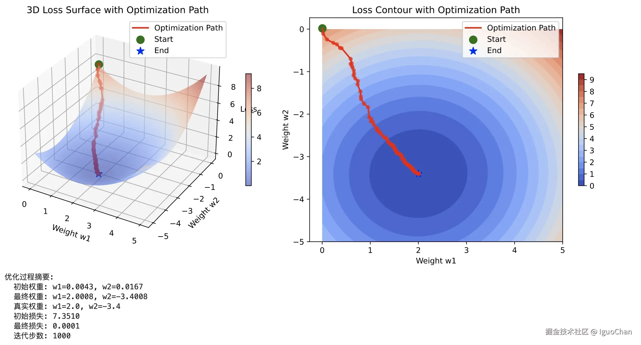
# 8. 打印优化过程摘要
print(f"优化过程摘要:")
print(f" 初始权重: w1={w_trajectory[0, 0]:.4f}, w2={w_trajectory[0, 1]:.4f}")
print(f" 最终权重: w1={w_trajectory[-1, 0]:.4f}, w2={w_trajectory[-1, 1]:.4f}")
print(f" 真实权重: w1={true_w[0]:.1f}, w2={true_w[1]:.1f}")
print(f" 初始损失: {trajectory_losses[0]:.4f}")
print(f" 最终损失: {trajectory_losses[-1]:.4f}")
print(f" 迭代步数: {len(w_trajectory)}")可以发现,当我们不考虑 b 的情形下,从任意起点开始,梯度下降会逐渐收缩到整个曲面的最低点附近,这也就使得梯度下降更易于理解了。