上一篇:【上海(1)】自行车数据协同路网、天气、区级数据解决问题--新手小白保姆级
十、 统计站点的流量
以二维坐标点为一个点。统计每个站点一个月内的总的借还车频次。3D柱状图表示。
1.数据读取和数据形状
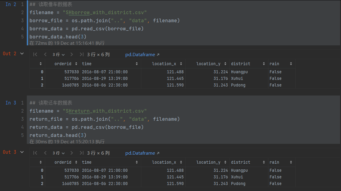
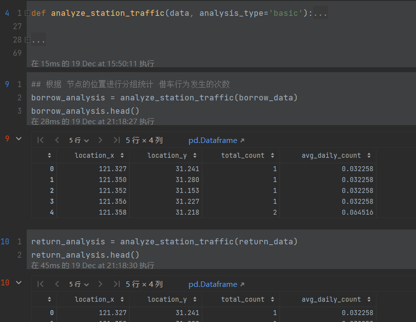
2. 根据节点的位置分组统计借车发生的次数
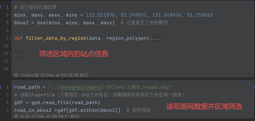
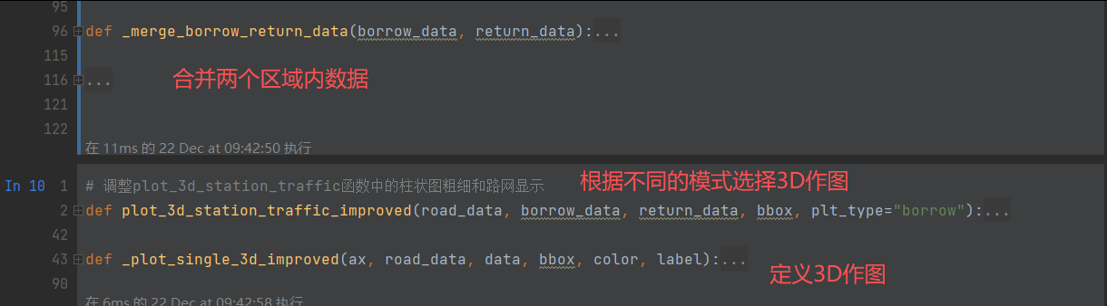
3. 筛选数据,画图
python
###########筛选区域内的路网和借还数据并生成含上海底图的柱状图---总执行代码#########
polygon_coords =  [(121.52, 31.22), (121.54, 31.22), (121.54, 31.23), (121.52, 31.23)]
bbox = Polygon(polygon_coords)

# road_path = "../shanghailuwang3-5files/上海市_roads.shp"
# gdf = gpd.read_file(road_path)
###路网筛选
road_in_bbox =gdf[gdf.within(bbox)]  # 矩形筛选

###borrow筛选
borrow_in_bbox= filter_data_by_region(borrow_analysis, bbox)

###return筛选
return_in_bbox=filter_data_by_region(return_analysis, bbox)

## 由于柱状图太多,还是无法看到地形图和柱状图的结合效果。现在我们筛选10条数据。
# 随机选择10个样本
borrow_10 = borrow_in_bbox.sample(n=10)
plot_3d_station_traffic_improved(road_in_bbox, borrow_10, return_in_bbox, bbox2, "borrow")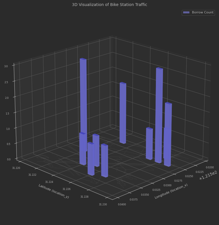
十一、Louvain算法
建立图并是用louvain算法进行社团检测
- 数据预处理与图构建
读取摩拜单车骑行数据文件 (mobike_shanghai_sample_updated.csv)
提取每条记录的起始点和终点坐标,构建有向边
计算边的权重(表示两点间骑行频次)
构建有向图 G,节点代表地理位置,边代表骑行路线 - 社区检测分析
使用Louvain算法对图进行社区检测
识别具有高内聚性的地理区域(社区)
统计社区数量和各社区节点分布情况 - 数据清洗与优化
识别并移除孤立节点(节点数量少于阈值的社区)
移除最左侧的异常节点
逐步生成优化后的图结构(图1、图2) - 可视化与结果输出
生成社区聚类图,展示不同社区的地理分布
保存图结构数据(节点和边信息)
保存各社区详细信息和统计数据
生成对比图展示清洗前后的社区分布变
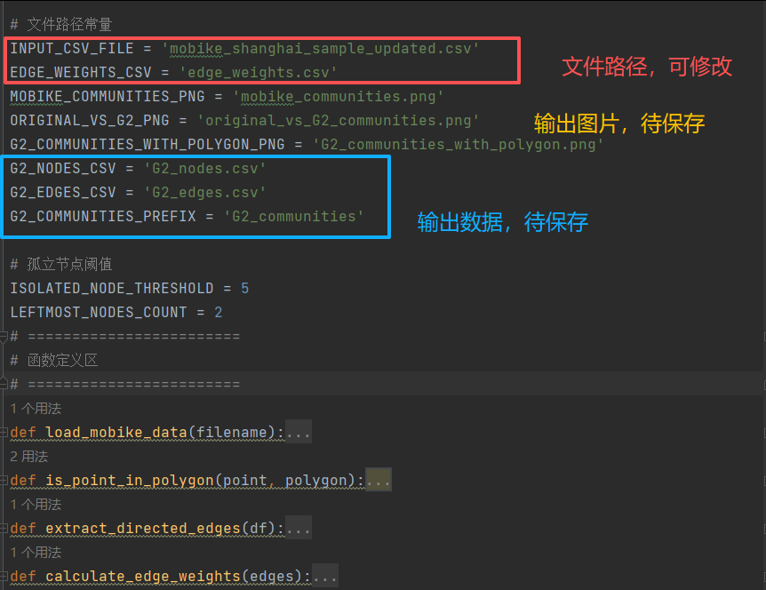
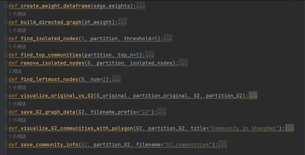
见代码dirEdge.py中
python
# 1. 读取数据文件
df = load_mobike_data(INPUT_CSV_FILE)
# 2. 提取起点和终点坐标,构建有向边
# 检查是否已存在edge_weights.csv文件
if os.path.exists(EDGE_WEIGHTS_CSV):
print(f"检测到已存在的 {EDGE_WEIGHTS_CSV} 文件,直接读取...")
df_weight = pd.read_csv(EDGE_WEIGHTS_CSV)
# 从df_weight重建edges列表(优化版)
edges = []
for _, row in df_weight.iterrows():
edge = (row['start_x'], row['start_y'], row['end_x'], row['end_y'])
# 只添加一次边,权重信息已在df_weight中保留
edges.append(edge)
else:
# 如果不存在则按原有流程处理
edges = extract_directed_edges(df)
# 3. 计算边的权重(出现频次)
edge_weights = calculate_edge_weights(edges)
# 4. 构建权重表格 df_weight
df_weight = create_weight_dataframe(edge_weights)
# 保存权重表格
df_weight.to_csv(EDGE_WEIGHTS_CSV, index=False)
print(f"已生成并保存 {EDGE_WEIGHTS_CSV} 文件")
# 5. 构建有向图
G = build_directed_graph(df_weight)
print(f"图中节点数量: {G.number_of_nodes()}")
print(f"图中边的数量: {G.number_of_edges()}")
print("前5条边的权重信息:")
print(df_weight.head())
# Louvain社团检测
try:
import community as community_louvain
# 将DiGraph转换为Graph进行社区检测
G_undirected = G.to_undirected()
# 应用Louvain算法进行社区检测
partition = community_louvain.best_partition(G_undirected)
# 将社区信息添加到节点属性
nx.set_node_attributes(G, partition, 'community')
print(f"检测到的社区数量: {len(set(partition.values()))}")
print("部分节点的社区分配:")
for i, (node, comm) in enumerate(list(partition.items())[:10]):
print(f"节点 {node}: 社区 {comm}")
except ImportError:
print("未安装python-louvain库,请运行: pip install python-louvain")
# 查找孤立的节点
isolated_nodes, all_community_sizes = find_isolated_nodes(G, partition, ISOLATED_NODE_THRESHOLD)
print(f"找到 {len(isolated_nodes)} 个孤立节点")
print("孤立节点列表(前10个):")
for node in list(isolated_nodes)[:10]:
print(f" 节点 {node}, 社区 {partition[node]}")
# 查找最大的5个社区
top_communities, all_community_sizes = find_top_communities(partition, top_n=5)
print("\n最大的5个社区:")
for comm_id, size in top_communities.items():
print(f" 社区 {comm_id}: {size} 个节点")
# 查看社区整体情况
print(f"\n社区总体情况:")
print(f" 总社区数: {len(all_community_sizes)}")
print(f" 平均社区大小: {sum(all_community_sizes.values()) / len(all_community_sizes):.2f}")
print(f" 最大社区: {max(all_community_sizes.values())} 个节点")
print(f" 最小社区: {min(all_community_sizes.values())} 个节点")
# 获取原始图中最左侧的两个节点
original_leftmost_nodes = find_leftmost_nodes(G, LEFTMOST_NODES_COUNT)
print(f"原始图中最左侧的两个节点: {original_leftmost_nodes}")
# 1. 删除所有的孤立节点,得到图1
G1 = G.copy()
G1.remove_nodes_from(isolated_nodes)
partition_G1 = {node: comm for node, comm in partition.items() if node not in isolated_nodes}
print(f"\n图1信息:")
print(f" 节点数量: {G1.number_of_nodes()} (原 {G.number_of_nodes()})")
print(f" 边的数量: {G1.number_of_edges()} (原 {G.number_of_edges()})")
# 2. 寻找图1的最左侧两个节点,并输出位置信息
G1_leftmost_nodes = find_leftmost_nodes(G1, LEFTMOST_NODES_COUNT)
print(f"图1中最左侧的两个节点: {G1_leftmost_nodes}")
# 3. 删除图1的最左侧的两个节点,生成图2
G2 = G1.copy()
G2.remove_nodes_from(G1_leftmost_nodes)
partition_G2 = {node: comm for node, comm in partition_G1.items() if node not in G1_leftmost_nodes}
print(f"\n图2信息:")
print(f" 节点数量: {G2.number_of_nodes()} (图1 {G1.number_of_nodes()})")
print(f" 边的数量: {G2.number_of_edges()} (图1 {G1.number_of_edges()})")
# 4. 寻找图2的最左侧两个节点,并输出位置信息
G2_leftmost_nodes = find_leftmost_nodes(G2, LEFTMOST_NODES_COUNT)
print(f"图2中最左侧的两个节点: {G2_leftmost_nodes}")
# 对原图和图2进行社区检测
# 原图社区检测
G_undirected = G.to_undirected()
partition_original_detected = community_louvain.best_partition(G_undirected)
# 图2社区检测
G2_undirected = G2.to_undirected()
partition_G2_detected = community_louvain.best_partition(G2_undirected)
# 输出社区检测结果
print(f"\n原图社区检测结果:")
print(f" 社区数量: {len(set(partition_original_detected.values()))}")
# 查找原图最大的5个社区
original_community_sizes = {}
for node, comm in partition_original_detected.items():
original_community_sizes[comm] = original_community_sizes.get(comm, 0) + 1
sorted_original_communities = sorted(original_community_sizes.items(), key=lambda x: x[1], reverse=True)
print(" 最大的5个社区:")
for i, (comm_id, size) in enumerate(sorted_original_communities[:5]):
print(f" 社区 {comm_id}: {size} 个节点")
print(f"\n图2社区检测结果:")
print(f" 社区数量: {len(set(partition_G2_detected.values()))}")
# 查找图2最大的5个社区
G2_community_sizes = {}
for node, comm in partition_G2_detected.items():
G2_community_sizes[comm] = G2_community_sizes.get(comm, 0) + 1
sorted_G2_communities = sorted(G2_community_sizes.items(), key=lambda x: x[1], reverse=True)
print(" 最大的5个社区:")
for i, (comm_id, size) in enumerate(sorted_G2_communities[:5]):
print(f" 社区 {comm_id}: {size} 个节点")
# 执行可视化对比
visualize_original_vs_G2(G, partition_original_detected, G2, partition_G2_detected)
print("Find good graph by cleaned some nodes!")
# 保存图2数据
save_G2_graph_data(G2, "G2")
# 绘制并保存图2社团聚类图
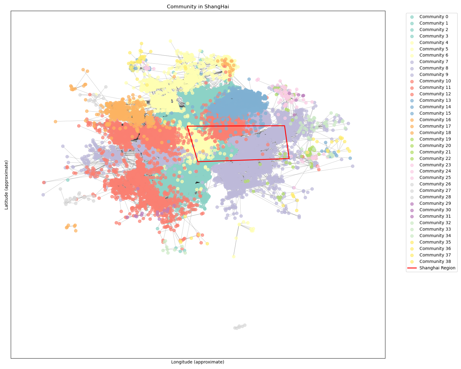
visualize_G2_communities_with_polygon(G2, partition_G2_detected, "Community in ShangHai")
# 保存图2社团信息
save_community_info(G2, partition_G2_detected, G2_COMMUNITIES_PREFIX)
print("已完成所有数据保存任务!")结果展示:
图中节点数量: 28557
图中边的数量: 94904
图2社区检测结果:
社区数量: 39
最大的5个社区:
社区 3: 3777 个节点
社区 9: 3261 个节点
社区 2: 2520 个节点
社区 5: 2134 个节点
社区 11: 1813 个节点
原数据社团检测VS删除异常点后社团检测
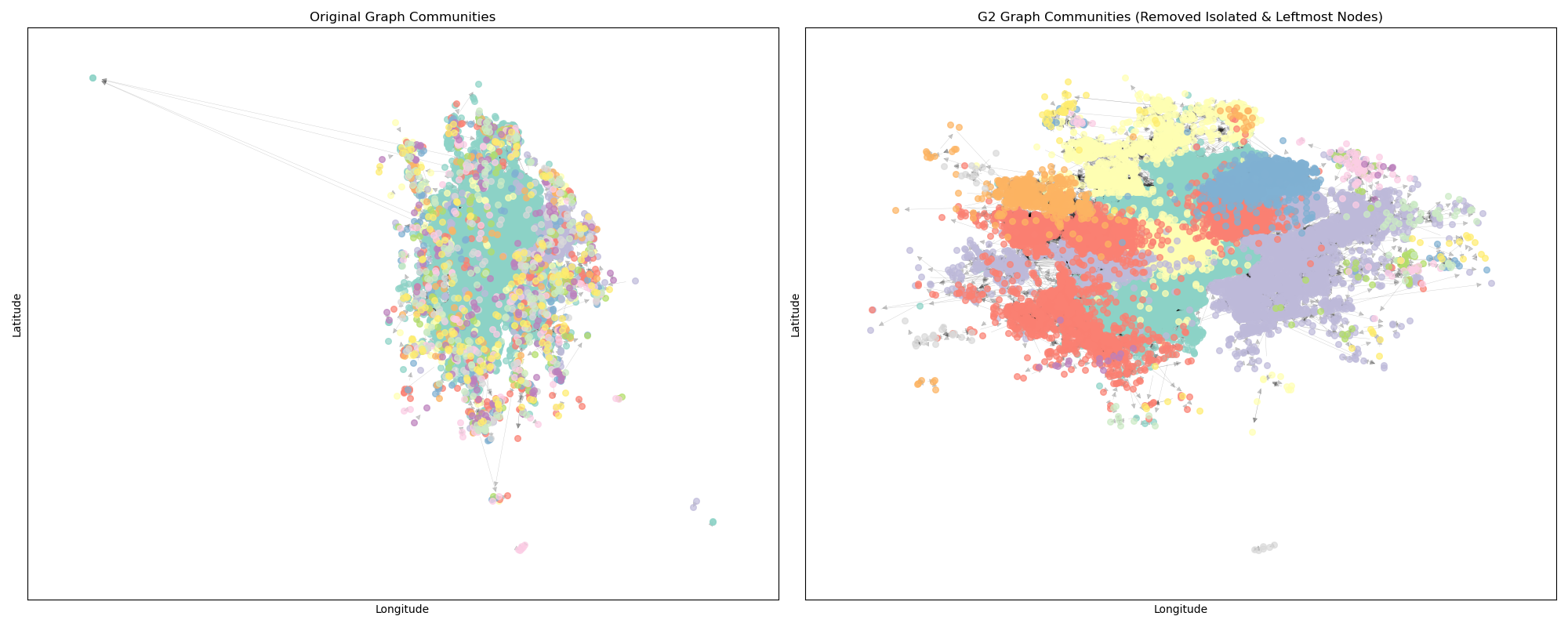
社团检测with区域标注
十二、流量统计
- 忽略站点属性、星期属性,查看以delta 为间隔的 流量/时间 频次折线图
- 选择某个社团,选择某个工作日或者某天,查看 流量/时间 频次折线图 。画 "潮汐"图 。
读取数据
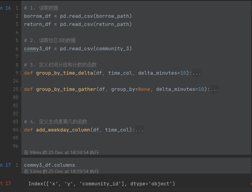
筛选数据
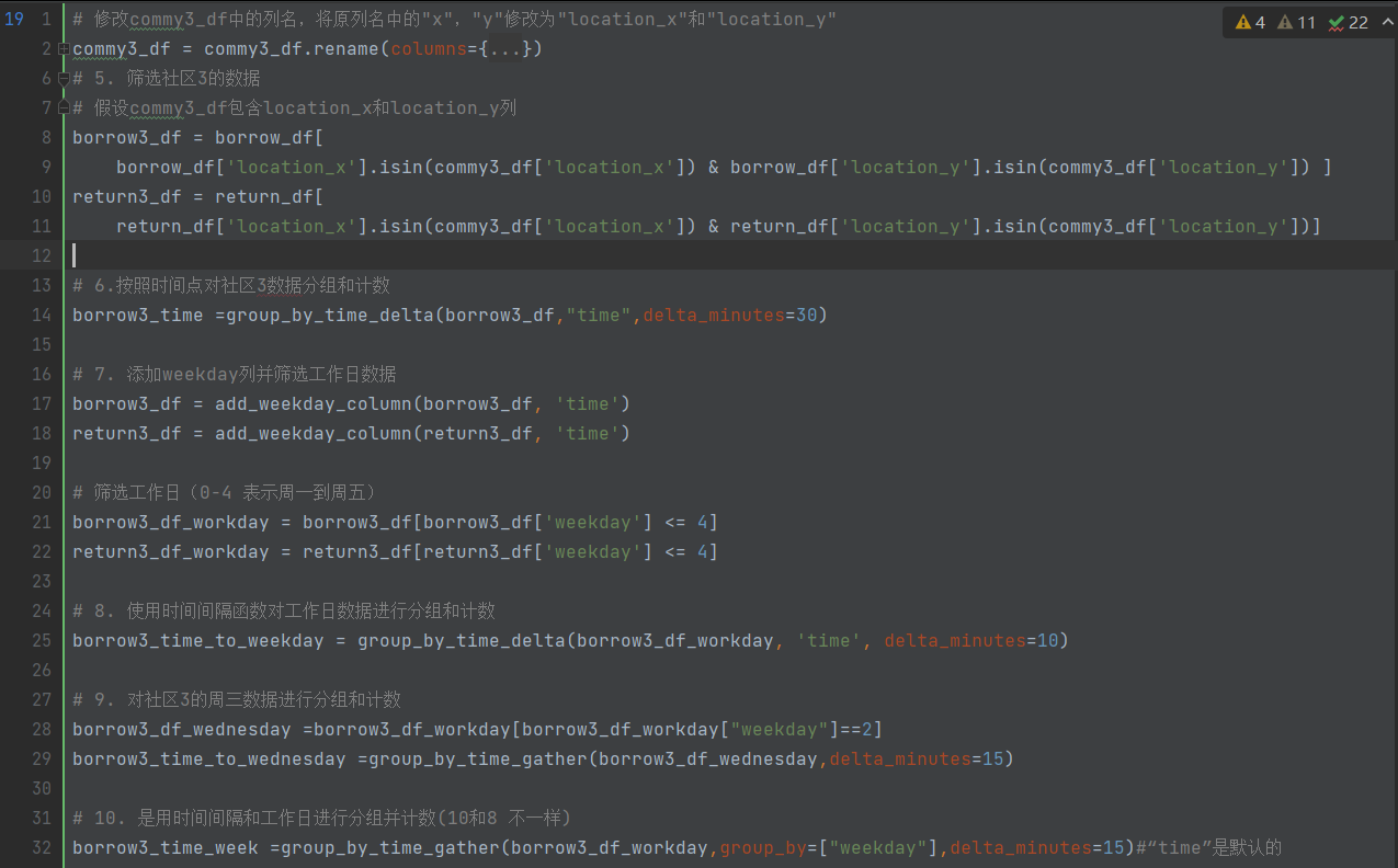
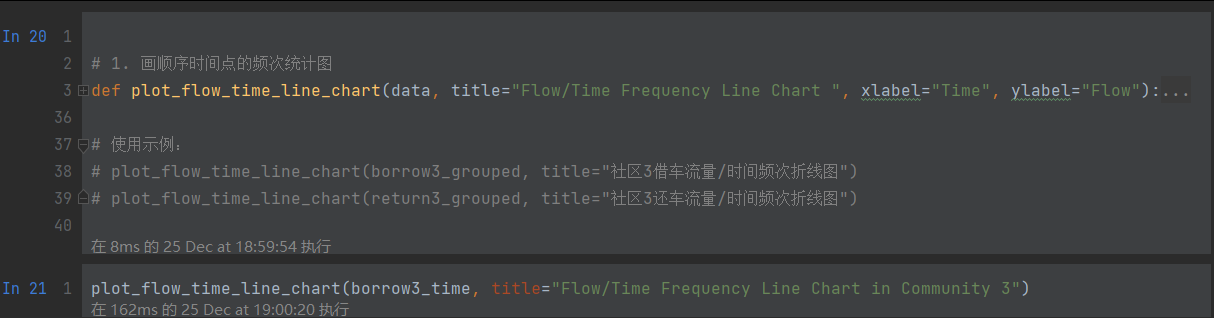
画图
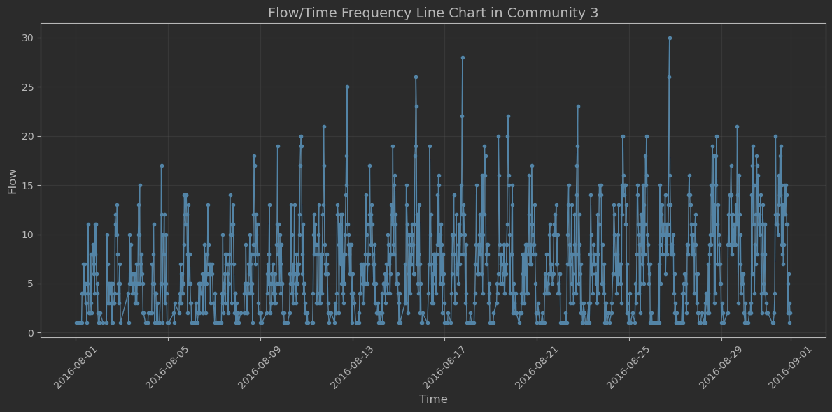
ps:以30分钟为间隔,统计了一个月时长的频次折线图。
python
plot_flow_time_line_chart(borrow3_time_to_wednesday,
title="Flow/Time Frequency Line Chart in Community 3 on Wednesday")
结果为:
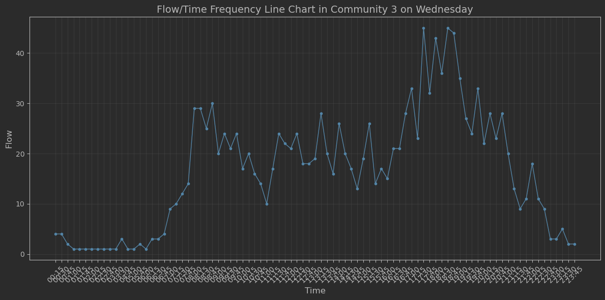
ps:选择了社区3星期三的借车频次图,以15分钟间隔统计。具有"潮汐现象"