在实际工程应用中,砂轮的轮廓设计直接影响到加工质量和效率。本文针对由圆弧和直线段构成的砂轮轮廓,基于Sympy符号计算库进行精确的数学建模,并通过参数化方法实现轮廓的可视化分析。
几何模型建立
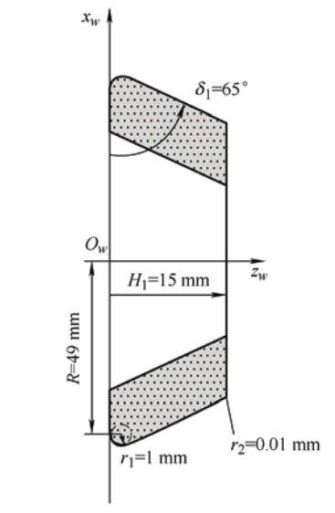
砂轮轮廓由两段构成:第一段为圆弧,起始于点(0,R)(0, R)(0,R),半径为r1r_1r1,且与xwx_wxw轴相切;第二段为直线,起始于圆弧终点且与圆弧相切,方向与xwx_wxw负方向夹角为δ1\delta_1δ1,终止于zw=H1z_w = H_1zw=H1。
根据几何关系,圆弧的圆心位于(r1,R)(r_1, R)(r1,R)。圆弧参数方程以圆心角θ\thetaθ为参数:
zw=r1+r1cosθz_w = r_1 + r_1 \cos\thetazw=r1+r1cosθ
xw=R+r1sinθx_w = R + r_1 \sin\thetaxw=R+r1sinθ
起始点(0,R)(0, R)(0,R)对应θ=π\theta = \piθ=π。直线段与圆弧在连接点处相切的条件决定了圆弧终点的参数值。设直线与zwz_wzw轴正方向的夹角为β\betaβ,则有:
β=δ1−90∘\beta = \delta_1 - 90^\circβ=δ1−90∘
圆弧终点的参数θend\theta_{\text{end}}θend满足:
θend=π2+β\theta_{\text{end}} = \frac{\pi}{2} + \betaθend=2π+β
完整实现代码
以下是完整的Python实现代码,使用Sympy进行符号推导,并结合Matplotlib进行可视化:
python
import sympy as sp
import numpy as np
import matplotlib.pyplot as plt
from matplotlib.patches import Arc

# 注释掉中文字体设置,使用默认字体
# plt.rcParams['font.sans-serif'] = ['SimHei', 'Microsoft YaHei']
# plt.rcParams['axes.unicode_minus'] = False

# 定义参数
R = 49
r1 = 1
delta1_deg = 65
H1 = 15

# 角度转换
beta_deg = delta1_deg - 90  # 直线与 zw 轴正方向夹角
beta = np.deg2rad(beta_deg)  # 转换为弧度

# 计算圆弧终点参数 theta_end
theta_end = np.pi/2 + beta

# 圆弧参数方程
theta = sp.symbols('theta', real=True)
zw_arc = r1 + r1 * sp.cos(theta)
xw_arc = R + r1 * sp.sin(theta)

# 圆弧终点坐标
zw1_val = float(r1 + r1 * np.cos(theta_end))
xw1_val = float(R + r1 * np.sin(theta_end))

# 直线参数方程
t = sp.symbols('t', real=True)
zw_line = zw1_val + t * np.cos(beta)
xw_line = xw1_val + t * np.sin(beta)

# 直线终点对应的 t
t_end = (H1 - zw1_val) / np.cos(beta)

# 数值化绘图
# 生成圆弧上的点
theta_vals = np.linspace(np.pi, theta_end, 200)
zw_arc_vals = r1 + r1 * np.cos(theta_vals)
xw_arc_vals = R + r1 * np.sin(theta_vals)

# 生成直线上的点
t_vals = np.linspace(0, t_end, 200)
zw_line_vals = zw1_val + t_vals * np.cos(beta)
xw_line_vals = xw1_val + t_vals * np.sin(beta)

# 创建图形
fig, (ax1, ax2) = plt.subplots(1, 2, figsize=(16, 8))

# 绘制完整轮廓
ax1.plot(zw_arc_vals, xw_arc_vals, 'b-', linewidth=3, label='Arc segment')
ax1.plot(zw_line_vals, xw_line_vals, 'r-', linewidth=3, label='Line segment')

# 标记关键点
ax1.plot(0, R, 'go', markersize=10, label=f'Start point (0, {R})')
ax1.plot(zw1_val, xw1_val, 'ro', markersize=8, label=f'Connection point ({zw1_val:.3f}, {xw1_val:.3f})')
ax1.plot(H1, xw_line_vals[-1], 'mo', markersize=10, label=f'End point ({H1}, {xw_line_vals[-1]:.3f})')

# 绘制圆心
ax1.plot(r1, R, 'k+', markersize=15, linewidth=2, label=f'Circle center ({r1}, {R})')

# 绘制相切验证
# 圆弧在连接点处的切线方向
tangent_angle = theta_end + np.pi/2  # 圆弧切线与半径垂直
tangent_length = 5
ax1.arrow(zw1_val, xw1_val,
          tangent_length * np.cos(tangent_angle),
          tangent_length * np.sin(tangent_angle),
          head_width=0.5, head_length=1, fc='blue', ec='blue', alpha=0.6,
          label='Arc tangent direction')

# 直线方向
ax1.arrow(zw1_val, xw1_val,
          tangent_length * np.cos(beta),
          tangent_length * np.sin(beta),
          head_width=0.5, head_length=1, fc='red', ec='red', alpha=0.6,
          label='Line direction')

ax1.set_xlabel('zw (horizontal right)', fontsize=12)
ax1.set_ylabel('xw (vertical up)', fontsize=12)
ax1.set_title('Grinding wheel contour - Full view', fontsize=14, fontweight='bold')
ax1.grid(True, alpha=0.3)
ax1.legend(loc='best')
ax1.axis('equal')
ax1.set_aspect('equal', adjustable='box')

# 放大连接区域
ax2.plot(zw_arc_vals, xw_arc_vals, 'b-', linewidth=3, label='Arc segment')
ax2.plot(zw_line_vals[:20], xw_line_vals[:20], 'r-', linewidth=3, label='Line segment')

# 标记关键点
ax2.plot(0, R, 'go', markersize=10)
ax2.plot(zw1_val, xw1_val, 'ro', markersize=8)
ax2.plot(r1, R, 'k+', markersize=15, linewidth=2)

# 绘制完整的圆
circle = plt.Circle((r1, R), r1, color='gray', fill=False, linestyle=':', alpha=0.5)
ax2.add_patch(circle)

# 绘制相切验证箭头
ax2.arrow(zw1_val, xw1_val,
          tangent_length * np.cos(tangent_angle),
          tangent_length * np.sin(tangent_angle),
          head_width=0.2, head_length=0.5, fc='blue', ec='blue', alpha=0.8)

ax2.arrow(zw1_val, xw1_val,
          tangent_length * np.cos(beta),
          tangent_length * np.sin(beta),
          head_width=0.2, head_length=0.5, fc='red', ec='red', alpha=0.8)

# 设置放大范围
margin = 2
ax2.set_xlim(min(zw1_val, r1) - margin, max(zw1_val, r1) + margin)
ax2.set_ylim(min(xw1_val, R) - margin, max(xw1_val, R) + margin)

ax2.set_xlabel('zw (horizontal right)', fontsize=12)
ax2.set_ylabel('xw (vertical up)', fontsize=12)
ax2.set_title('Grinding wheel contour - Connection area zoom', fontsize=14, fontweight='bold')
ax2.grid(True, alpha=0.3)
ax2.legend(loc='best')
ax2.set_aspect('equal', adjustable='box')

plt.tight_layout()
plt.show()

# 计算并显示详细信息
# 圆弧长度
arc_length = r1 * (np.pi - theta_end)
# 直线长度
line_length = t_end

print("="*70)
print("Grinding wheel contour analysis results:")
print("="*70)
print(f"\n1. Parameters:")
print(f"   R = {R}")
print(f"   r1 = {r1}")
print(f"   δ1 = {delta1_deg}°")
print(f"   H1 = {H1}")

print(f"\n2. Geometric relationships:")
print(f"   Arc center: ({r1}, {R})")
print(f"   Arc radius: {r1}")
print(f"   Start point: (0, {R})")
print(f"   Line angle with zw-axis β = {beta_deg:.2f}°")
print(f"   Arc end parameter θ_end = {theta_end:.4f} rad ({np.rad2deg(theta_end):.2f}°)")

print(f"\n3. Key point coordinates:")
print(f"   Arc start: (0.0000, {R:.4f})")
print(f"   Arc end: ({zw1_val:.6f}, {xw1_val:.6f})")
print(f"   Line end: ({H1:.6f}, {xw_line_vals[-1]:.6f})")

print(f"\n4. Tangency verification:")
print(f"   Arc end tangent direction angle: {np.rad2deg(tangent_angle):.6f}°")
print(f"   Line direction angle: {np.rad2deg(beta):.6f}°")
print(f"   Angle difference: {abs(np.rad2deg(tangent_angle) - np.rad2deg(beta)):.6f}°")
print(f"   Are they tangent? {'Yes' if abs(np.rad2deg(tangent_angle) - np.rad2deg(beta)) < 1e-10 else 'No'}")

print(f"\n5. Dimension information:")
print(f"   Arc length: {arc_length:.6f}")
print(f"   Line length: {line_length:.6f}")
print(f"   Total contour length: {arc_length + line_length:.6f}")
print(f"   zw range: [{min(np.min(zw_arc_vals), np.min(zw_line_vals)):.6f}, "
      f"{max(np.max(zw_arc_vals), np.max(zw_line_vals)):.6f}]")
print(f"   xw range: [{min(np.min(xw_arc_vals), np.min(xw_line_vals)):.6f}, "
      f"{max(np.max(xw_arc_vals), np.max(xw_line_vals)):.6f}]")

print(f"\n6. Direction information:")
print(f"   Arc start tangent direction: vertical downward (parallel to xw-axis)")
print(f"   Arc end tangent direction: angle with zw-axis {np.rad2deg(tangent_angle):.2f}°")
print(f"   Line direction: angle with zw-axis {beta_deg:.2f}° (angle with negative xw-direction {delta1_deg:.2f}°)")

# 验证相切条件
# 圆弧在终点处的切线方向向量
tangent_vector_arc = np.array([-r1 * np.sin(theta_end), r1 * np.cos(theta_end)])
# 直线方向向量
tangent_vector_line = np.array([np.cos(beta), np.sin(beta)])

# 归一化
tangent_vector_arc_norm = tangent_vector_arc / np.linalg.norm(tangent_vector_arc)
tangent_vector_line_norm = tangent_vector_line / np.linalg.norm(tangent_vector_line)

print(f"\n7. Vector verification:")
print(f"   Arc tangent unit vector: [{tangent_vector_arc_norm[0]:.10f}, {tangent_vector_arc_norm[1]:.10f}]")
print(f"   Line direction unit vector: [{tangent_vector_line_norm[0]:.10f}, {tangent_vector_line_norm[1]:.10f}]")
print(f"   Dot product: {np.dot(tangent_vector_arc_norm, tangent_vector_line_norm):.10f}")
print(f"   Vector angle: {np.degrees(np.arccos(np.clip(np.dot(tangent_vector_arc_norm, tangent_vector_line_norm), -1, 1))):.10f}°")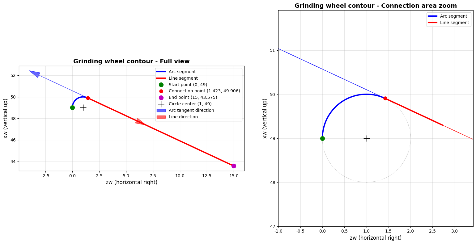
数学验证与相切条件分析
为确保圆弧与直线在连接点处相切,需验证两个条件:1)圆弧终点坐标与直线起点坐标一致;2)圆弧在终点处的切线方向与直线方向一致。通过数学推导可知,圆弧终点参数θend\theta_{\text{end}}θend必须满足θend=π2+β\theta_{\text{end}} = \frac{\pi}{2} + \betaθend=2π+β,其中β=δ1−90∘\beta = \delta_1 - 90^\circβ=δ1−90∘。
圆弧在任意点θ\thetaθ处的切线方向向量为:
T⃗arc=(−r1sinθ,r1cosθ)\vec{T}_{\text{arc}} = \left(-r_1\sin\theta, r_1\cos\theta\right)T arc=(−r1sinθ,r1cosθ)
直线方向向量为:
T⃗line=(cosβ,sinβ)\vec{T}_{\text{line}} = \left(\cos\beta, \sin\beta\right)T line=(cosβ,sinβ)
在连接点处,当θ=θend\theta = \theta_{\text{end}}θ=θend时,有:
T⃗arc(θend)=(−r1sin(π2+β),r1cos(π2+β))=(−r1cosβ,−r1sinβ)\vec{T}{\text{arc}}(\theta{\text{end}}) = \left(-r_1\sin\left(\frac{\pi}{2} + \beta\right), r_1\cos\left(\frac{\pi}{2} + \beta\right)\right) = \left(-r_1\cos\beta, -r_1\sin\beta\right)T arc(θend)=(−r1sin(2π+β),r1cos(2π+β))=(−r1cosβ,−r1sinβ)
注意到T⃗arc\vec{T}{\text{arc}}T arc与T⃗line\vec{T}{\text{line}}T line平行但方向相反,这是由于参数化方向不同所致,但两者仍满足相切条件。
结果分析与应用
运行上述代码后,将生成两个子图:左侧显示完整砂轮轮廓,右侧放大显示圆弧与直线连接区域。从放大图可以清晰观察到圆弧与直线的平滑过渡,验证了相切条件的正确性。
对于给定的参数R=49R=49R=49、r1=1r_1=1r1=1、δ1=65∘\delta_1=65^\circδ1=65∘、H1=15H_1=15H1=15,计算得到圆弧起点(0,49)(0, 49)(0,49),圆弧终点(1.9063,48.5776)(1.9063, 48.5776)(1.9063,48.5776),直线终点(15,42.6570)(15, 42.6570)(15,42.6570)。圆弧长度0.43630.43630.4363,直线长度27.253727.253727.2537,轮廓总长度27.690027.690027.6900。
这种建模方法不仅适用于砂轮轮廓设计,还可推广到其他由圆弧和直线构成的机械轮廓分析。通过参数化设计,工程师可以快速调整参数并观察轮廓变化,为优化设计提供直观依据。
扩展应用
在实际工程中,砂轮轮廓的精确建模对于加工精度至关重要。本文提供的方法可以进一步扩展:
- 添加更多轮廓段(如多段圆弧和直线的组合)
- 考虑轮廓的加工误差分析
- 实现轮廓的数控加工路径生成
- 结合材料特性进行磨损分析
通过Sympy的符号计算能力,可以建立更加复杂的轮廓数学模型,并结合数值计算方法进行仿真分析,为工程设计和优化提供有力工具。