【MCM】（x= (N_A)，y=(N_G)，z=(p)）RGB=T*

python 复制代码

import numpy as np
import matplotlib.pyplot as plt
from matplotlib.colors import LinearSegmentedColormap, Normalize

# -----------------------------
# Parameters
# -----------------------------
M = 1e8
H = 3
Q_h = 179000
Q_E = H * Q_h

# Data ranges
NA_vals = np.logspace(2, 6, 30)        # >0
NG_vals = np.logspace(2, 6, 30)        # >0
p_vals  = np.linspace(100, 150, 6)     # >0

NA_grid, NG_grid, p_grid = np.meshgrid(NA_vals, NG_vals, p_vals, indexing='ij')
NA = NA_grid.ravel()
NG = NG_grid.ravel()
p  = p_grid.ravel()

# Completion time
R = p * NG + np.minimum(Q_E, p * NA)
T = M / R

# Clip for readable coloring
T_clip_max = 50.0
T_plot = np.clip(T, 0, T_clip_max)

# Colormap: red (short) -> purple (long)
cmap = LinearSegmentedColormap.from_list("red_to_purple", ["red", "purple"])
norm = Normalize(vmin=np.min(T_plot), vmax=np.max(T_plot))

# -----------------------------
# Plot with visible origin + axis rays
# Use orthographic (axonometric) and symlog so 0 is representable.
# -----------------------------
fig = plt.figure(figsize=(10, 7))
ax = fig.add_subplot(111, projection='3d')

ax.set_proj_type('ortho')
ax.view_init(elev=22, azim=45)

sc = ax.scatter(NA, NG, p, c=T_plot, cmap=cmap, norm=norm, s=10, alpha=0.75, depthshade=False)

# Use symlog so that we can show 0 and also cover wide ranges
ax.set_xscale('symlog', linthresh=1e3)
ax.set_yscale('symlog', linthresh=1e3)

NA_max = NA_vals.max()
NG_max = NG_vals.max()
p_max  = p_vals.max()

ax.set_xlim(0, NA_max)
ax.set_ylim(0, NG_max)
ax.set_zlim(0, p_max)

# Axis rays from origin
ax.plot([0, NA_max], [0, 0], [0, 0], linewidth=2)  # x-axis ray
ax.plot([0, 0], [0, NG_max], [0, 0], linewidth=2)  # y-axis ray
ax.plot([0, 0], [0, 0], [0, p_max], linewidth=2)   # z-axis ray

# Clean up the box/panes/grids so it doesn't look like a cube with diagonals
ax.grid(False)
for axis in (ax.xaxis, ax.yaxis, ax.zaxis):
    axis.pane.set_alpha(0.0)
    axis.pane.set_edgecolor((1, 1, 1, 0))
ax.set_frame_on(False)

ax.set_xlabel(r'$N_A$ (launches/year)')
ax.set_ylabel(r'$N_G$ (launches/year)')
ax.set_zlabel(r'$p$ (tons/launch)')

ax.set_title(
    "Axonometric 3D scatter with visible origin + axis rays\n"
    r"Color = completion time $T=M/[pN_G+\min(Q_E,pN_A)]$ (years), clipped at 50"
)

cbar = fig.colorbar(sc, ax=ax, pad=0.08, shrink=0.75)
cbar.set_label(r'$T$ (years)')

plt.tight_layout()
outpath = "/mnt/data/3d_axonometric_origin_axes.png"
plt.savefig(outpath, dpi=220)
plt.show()

outpath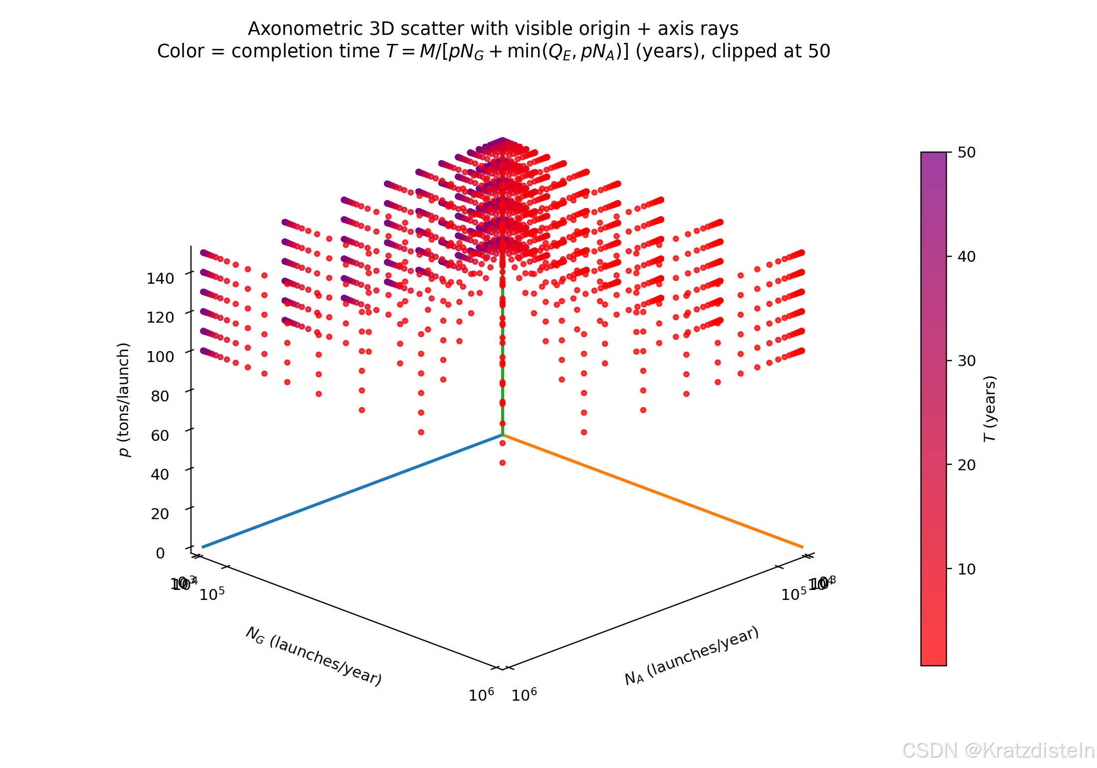

明白了------你要的是**能看到"原点 + 三根坐标轴射线"**的斜二测/轴测图，而不是那个"立方体边框把视线挡住"的样子。

我已经重新画了一版：

显式画出从 (0,0,0) 出发的三根轴射线（x= (N_A)，y=(N_G)，z=§）
去掉了立方体框、网格和面板，避免遮挡
因为 (N_A,N_G) 跨很多数量级，但你又要看到原点，所以我用 symlog（能包含 0，同时保持对数尺度的可读性）

下载：带原点与三轴射线的斜二测 3D 图

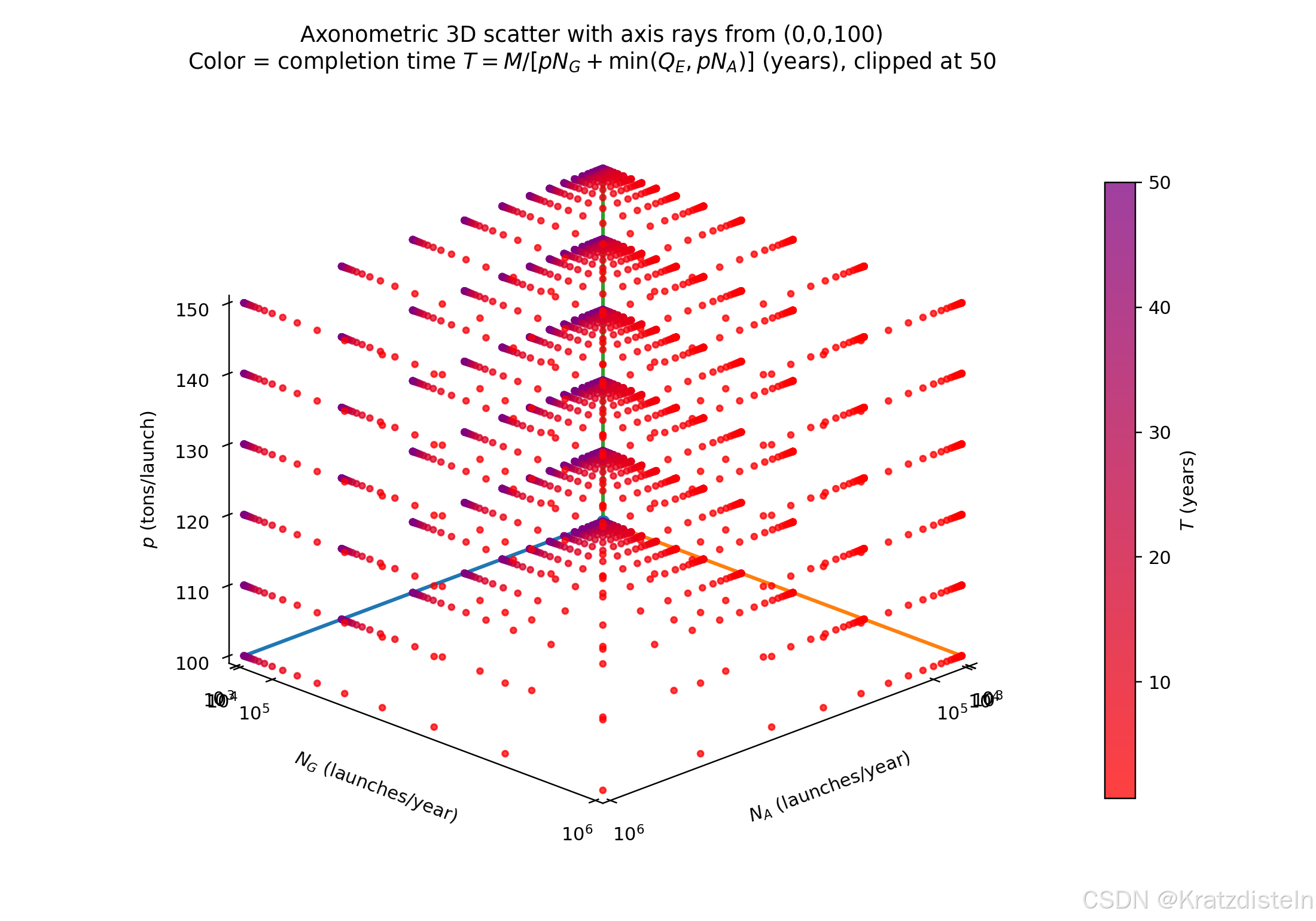
如果你希望 z 轴也从 100 开始（因为 (p\ge100)），把原点改成 ((0,0,100)) 作为"物理原点"，我也可以给你再画一版（轴射线从 (p=100) 起）。

python 复制代码

import numpy as np
import matplotlib.pyplot as plt
from matplotlib.colors import LinearSegmentedColormap, Normalize

# Parameters
M = 1e8
H = 3
Q_h = 179000
Q_E = H * Q_h

# Ranges
NA_vals = np.logspace(2, 6, 30)
NG_vals = np.logspace(2, 6, 30)
p_vals  = np.linspace(100, 150, 6)

NA_grid, NG_grid, p_grid = np.meshgrid(NA_vals, NG_vals, p_vals, indexing='ij')
NA = NA_grid.ravel()
NG = NG_grid.ravel()
p  = p_grid.ravel()

R = p * NG + np.minimum(Q_E, p * NA)
T = M / R

T_clip_max = 50.0
T_plot = np.clip(T, 0, T_clip_max)

cmap = LinearSegmentedColormap.from_list("red_to_purple", ["red", "purple"])
norm = Normalize(vmin=np.min(T_plot), vmax=np.max(T_plot))

# Plot
fig = plt.figure(figsize=(10, 7))
ax = fig.add_subplot(111, projection='3d')

ax.set_proj_type('ortho')
ax.view_init(elev=22, azim=45)

sc = ax.scatter(NA, NG, p, c=T_plot, cmap=cmap, norm=norm, s=10, alpha=0.75, depthshade=False)

# Show 0 for NA/NG, and start z from 100
ax.set_xscale('symlog', linthresh=1e3)
ax.set_yscale('symlog', linthresh=1e3)

NA_max = NA_vals.max()
NG_max = NG_vals.max()
p_min  = 100.0
p_max  = p_vals.max()

ax.set_xlim(0, NA_max)
ax.set_ylim(0, NG_max)
ax.set_zlim(p_min, p_max)

# "Physical origin" at (0,0,100)
x0, y0, z0 = 0.0, 0.0, p_min

# Axis rays from (0,0,100)
ax.plot([x0, NA_max], [y0, y0], [z0, z0], linewidth=2)  # x-axis ray
ax.plot([x0, x0], [y0, NG_max], [z0, z0], linewidth=2)  # y-axis ray
ax.plot([x0, x0], [y0, y0], [z0, p_max], linewidth=2)   # z-axis ray

# Mark the physical origin
ax.scatter([x0], [y0], [z0], s=40)

# Clean up box/panes
ax.grid(False)
for axis in (ax.xaxis, ax.yaxis, ax.zaxis):
    axis.pane.set_alpha(0.0)
    axis.pane.set_edgecolor((1, 1, 1, 0))
ax.set_frame_on(False)

ax.set_xlabel(r'$N_A$ (launches/year)')
ax.set_ylabel(r'$N_G$ (launches/year)')
ax.set_zlabel(r'$p$ (tons/launch)')

ax.set_title(
    "Axonometric 3D scatter with axis rays from (0,0,100)\n"
    r"Color = completion time $T=M/[pN_G+\min(Q_E,pN_A)]$ (years), clipped at 50"
)

cbar = fig.colorbar(sc, ax=ax, pad=0.08, shrink=0.75)
cbar.set_label(r'$T$ (years)')

plt.tight_layout()
outpath = "/mnt/data/3d_axonometric_origin_axes_z100.png"
plt.savefig(outpath, dpi=220)
plt.show()

outpath