注:本文为 "CPU 缓存" 相关合辑。
英文引文,机翻未校。
中文引文,略作重排。
如有内容异常,请看原文。
What is cache memory - Gary explains
什么是高速缓存------盖里科普讲解
By April 7, 2016
发布于 2016 年 04 月 07 日
SoC designers have a problem: RAM is slow and it can't keep up with the CPU. The workaround is known as cache memory. If you want to know all about cache memory then read on!
片上系统研发人员面临一项难题:随机存取存储器读写速率偏低,无法匹配中央处理器运行速度,高速缓存便是该问题的解决方案。想要全面了解高速缓存相关知识,请继续阅读下文。
System-on-a-Chip (SoC) designers have a problem, a big problem in fact, Random Access Memory (RAM) is slow, too slow, it just can't keep up. So they came up with a workaround and it is called cache memory. If you want to know all about cache memory then read on!
片上系统(SoC)设计者面临棘手难题:随机存取存储器(RAM)运行速率过慢,跟不上处理器运算节奏,研发人员由此设计出高速缓存作为折中方案,想要深入了解高速缓存,请继续浏览正文。
You may think it strange to hear that RAM is slow, you might have heard that hard disks are slow, CDROMs are slow, but main memory, are you serious? Of course, speed is relative. We might say that a certain type of road car is the fastest, but then it is relatively slow when compared to a Formula 1 racing car, which itself is slow compared to a supersonic jet and so on.
听到主存运行速度偏慢的说法或许会让人费解,大众通常只知晓硬盘、光盘驱动器读写迟缓,很难理解主存也存在速率短板。运行速度本身是相对概念,好比某款量产民用轿车在民用车型里提速最快,但对比一级方程式赛车就略显迟缓,而赛车相较于超音速喷气飞机又存在速度差距,以此类推。
At the heart of a System-on-a-Chip is the CPU. It rules supreme and it is very demanding. The average mobile CPU is clocked at anywhere from 1.5 GHz to around 2.2GHz. But the average RAM module is clocked at just 200MHz. So what that means is that the average bank of RAM is running with a clock speed that is a factor of 10 slower. For the CPU this is an eon. When it requests something from RAM it has to wait and wait and wait while the data is fetched, time in which it could be doing something else, but can't as it needs to wait...
中央处理器是片上系统的核心器件,运算效率高、对数据供给速率要求严苛。移动端主流处理器主频区间为 1.5 GHz ~ 2.2 GHz,而常规内存模组的工作主频仅为 200 MHz,内存时钟速率约为处理器的十分之一。对处理器而言,等待内存回传数据的耗时极其漫长;处理器发起内存读取请求后,只能搁置后续运算持续等待数据加载。
OK, I will admit, that is a bit of an over simplification, however it does show us the heart of the problem. The situation isn't actually that bad because of technologies like Double-Data-Rate (DDR) RAM which can send data twice per clock cycle. Likewise specifications like LPDDR3 (Low Power DDR3) allow for a data transfer rate eight times that of the internal clock. There are also techniques which can be built into the CPU which ensure that the data is requested as early as possible, before it is actually needed.
上述内容做了适度简化,但精准点明速率矛盾的本源。得益于双倍数据速率(DDR)内存等技术优化,实际硬件工况没有如此极端:DDR 内存可在单个时钟周期完成两次数据收发;低功耗第三代双倍速率内存(LPDDR3)的数据传输速率可达芯片内部时钟速率的八倍。此外处理器内部集成预取技术,可在程序实际取用数据前提前发起内存读取请求。
At the time of writing the latest SoCs are using [LPDDR4 with an effective speed of 1866MHz, so if the CPU is clocked at 1.8GHz or less the memory should keep up, or does it? The problem is that modern processors uses 4 or 8 CPU cores, so there isn't just one CPU trying to access the memory, there are 8 of them and they all want that data, and they want it ASAP!
本文撰稿时,新一代片上系统普遍搭载有效工作频率为 1866 MHz 的 LPDDR4 内存,单颗主频 1.8 GHz 及以下的处理器理论上可以匹配内存速率。但现代处理器普遍集成 4 核或 8 核运算单元,多核心会同时并发访问内存,所有内核都需要即时获取所需数据。
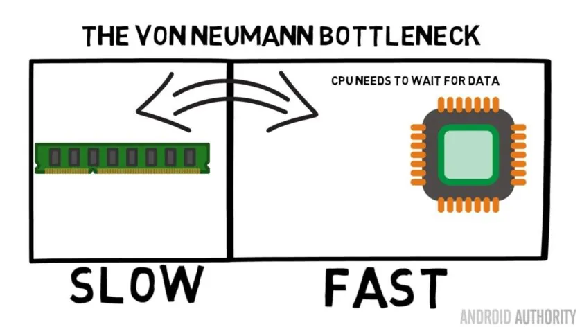
This performance limitation is known as the Von Neumann bottleneck. If you watched my [assembly language and machine code video you will remember that Von Neumann was one of the key people in the invention of the modern day computer. The downside of the Von Neumann architecture is the performance bottleneck which appears when the data throughput is limited due to the relative speed differences between the CPU and the RAM.
该类性能约束被称作冯·诺依曼瓶颈。看过我汇编与机器码科普视频的读者应当了解,冯·诺依曼是现代计算机体系的奠基人之一。冯·诺依曼架构的短板在于:处理器与内存的运行速率落差会限制整机数据吞吐能力,进而形成性能瓶颈。
There are some methods to improve this situation and decrease the performance differential, one of which is the use of cache memory. So what is cache memory? Put simply it is a small amount of memory that is built into the SoC that runs at the same speed as the CPU. This means that the CPU doesn't need to wait around for data from the cache memory, it is sent over to the CPU at the same speed that the CPU operates. Moreover the cache memory is installed on a per CPU core basis, that means that each CPU core has its own cache memory and there won't be any contention about who gets access to it.
现有多种优化方案可以缩小处理器与内存的性能差距,高速缓存便是其中之一。简单来说,高速缓存是集成在片上系统内部的小容量存储单元,运行主频与处理器完全同步。处理器读取缓存内数据时无需等待,数据传输速率和处理器运算速率保持一致。高速缓存按处理器内核独立配置,每颗核心独享专属缓存,不会出现多核心抢占缓存资源的冲突。
I can hear you thinking it now, why not make all memory like cache memory? The answer is simply, cache memory that runs at that speed is very expensive. Price (and to some extent the limitations of the fabrication technology) is a real barrier, that is why on mobile the average amount of cache memory is measured in Kilobytes, maybe 32K or 64K.
想必读者会产生疑问:为何不把全部内存都做成缓存规格?答案很直观:同频高速存储的制造成本高昂,生产成本与芯片制造工艺上限约束了缓存容量,移动端处理器的单核心缓存容量通常仅为千字节级别,常见规格为 32 K、64 K。
So, each CPU core has a few Kilobytes of super fast memory which it can use to store a copy of some of the main memory. If the copy in the cache is actually the memory that the CPU needs then it doesn't need to access the "slow" main memory to get the data. Of course, the trick is making sure that the memory in the cache is the best, the optimal, data so that the CPU can use the cache more and the main memory less.
每颗处理器内核配备数 KB 的高速存储空间,用于存放主存数据副本。当处理器所需数据已存入缓存副本时,就不必访问低速主存读取数据。缓存优化的核心思路,就是尽可能在缓存中留存处理器高频访问的数据,提升缓存取用占比、减少主存访问频次。
Since it only has a few Kilobytes of cache memory available there will be times when the cache has the right memory contents, known as a hit, and times when it doesn't, known as a miss. The more cache hits the better.
受限于缓存仅有数 KB 的可用空间,数据请求分为两种结果:所需数据已存放在缓存中称为缓存命中,数据不在缓存内称为缓存缺失,缓存命中次数越高整机性能越优。
Split caches and hierarchy
分离式缓存与缓存分级架构
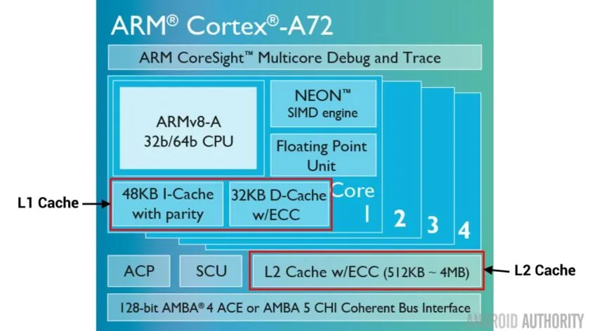
To help improve the number of hits versus misses there are a number of techniques which are used. One is to divide the cache in two, one for instructions and one for data. The reason to do this is that filling an instruction cache is much easier, since the next instruction to be executed is probably the next instruction in the memory. It also means that the next instruction to be executed can be fetched from the instruction cache while the CPU is also working on memory in the data cache (since the two caches are independent).
业内采用多项优化手段提升缓存命中率,分离式缓存是其中一种方案:将缓存拆分为指令缓存、数据缓存两个独立区块。程序指令具备顺序执行的特征,后续待运行指令大多在内存中紧邻排布,指令缓存的数据预填充难度更低;两类缓存相互独立,处理器在数据缓存中运算的同时,可从指令缓存预读取下一条程序指令。
Another technique to improve overall cache hits is to use a hierarchy of caches, these are traditionally known as L1 (level 1) and L2 (level 2) caches. L2 is normally a much larger cache, in the Megabyte range (say 4MB, but it can be more), however it is slower (meaning it cheaper to make) and it services all the CPU cores together, making it a unified cache for the whole SoC.
缓存分级架构是另一项提升全局命中率的方案,主流划分为一级缓存(L1)与二级缓存(L2)。二级缓存容量更大,容量多在兆字节区间(典型规格 4 MB,也可按需扩容),运行主频低于一级缓存、制造成本更低,作为片上系统共用缓存为全部处理器内核提供数据服务。
The idea is that if the requested data isn't in the L1 cache then the CPU will try the L2 cache before trying main memory. Although the L2 is slower than the L1 cache it is still faster than the main memory and due to its increased size there is a higher chance that the data will be available. Some chip designs also use a L3 cache. Just as L2 is slower but larger than L1, so L3 is slower but larger than L2. On mobile L3 cache isn't used, however ARM based processors which are used for servers (like the upcoming [24-core Qualcomm server SoC or the AMD Opteron 1100) have the option of adding a 32MB L3 cache.
数据查找优先级依次为一级缓存、二级缓存、主存;若一级缓存未命中,处理器转向二级缓存检索数据。二级缓存速率不及一级缓存,但远优于主存,更大的容量也提升了数据命中概率。部分芯片方案额外搭载三级缓存(L3),三级缓存相较二级缓存容量更大、运行速率更低。移动端处理器基本不配置三级缓存,面向服务器的 ARM 架构处理器(例如即将量产的高通 24 核服务器片上系统、AMD 皓龙 1100 系列)可选配 32 MB 规格三级缓存。
Associativity
缓存相联映射机制
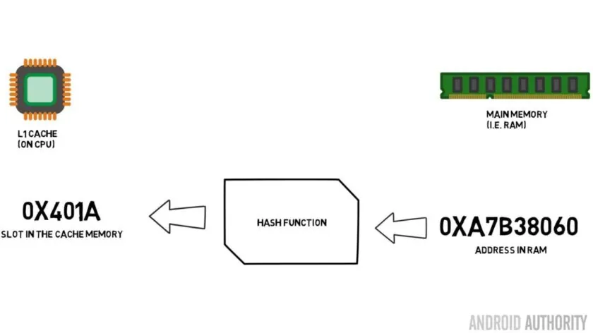
There is one more piece in the cache memory jigsaw. How does the CPU know where the contents from main memory is stored in the cache? If the cache was just a long list (a table) of cached memory slots then the CPU would need to search that list from top to bottom to find the contents it needs. That, of course, would be slower than fetching the contents from main memory. So to make sure that the memory contents can be found quickly a technique known as hashing needs to be used.
缓存体系还有关键一环:处理器如何定位主存数据在缓存中的存放位置?倘若缓存只是线性排布的存储列表,处理器需要自上而下全表检索目标数据,该检索耗时甚至高于直接读取主存。哈希映射算法被引入缓存设计,用来实现数据的快速寻址。
A hash function takes a value (in this case the address of the memory contents being mirrored in the cache) and generates a value for it. The same address always generates the same hash value. So the way the cache would work is that the address is hashed and it gives a fixed answer, an answer that fits within the size of the cache, i.e. 32K). Since 32K is much smaller than the size of RAM, the hash needs to loop, which means that after 32768 addresses the hash will give the same result again. This is known as direct mapping.
哈希函数接收输入值(本场景为待缓存的主存地址)并生成固定哈希结果,相同内存地址永远对应同一个哈希值。缓存通过地址哈希运算得到落在缓存容量区间(例如 32 K)内的存储下标;由于缓存空间远小于主存总容量,哈希结果会周期性循环,每间隔 32768 个地址就会出现哈希值重复,该映射方式称作直接映射。
The downside of this approach can be seen when the contents of two addresses need to be cached but the two addresses return the same cache slot (i.e. they have the same hash value). In such situations only one of the memory locations can be cached and the other remains only in main memory.
直接映射存在明显缺陷:两个不同内存地址经哈希运算指向同一个缓存槽位时,仅有一份数据可存入缓存,另一份数据只能留存于主存,无法被缓存。
Another approach is to use a hash which works in pairs, so any address can be one of a pair of locations in the cache, i.e. hash and hash +1. This means that two addresses which previously would have clashed, as they had the same hash, can now co-exist. But to find the right slot in the cache the CPU needs to check 2 locations, however that is still much faster than searching 32768 possible locations! The technical name for this mapping is called 2-way associative. The associative approach can be extended to 4-way, 8-way, and 16-way, however there are limits where the performance gains don't warrant the extra complexity or costs.
二路相联映射优化了哈希冲突问题:单个哈希下标对应一组两个缓存位置(哈希下标、哈希下标+1),原本哈希冲突的两个地址可分别存入一组内的两个槽位。处理器寻址时最多遍历 2 个存储位置,对比全量遍历 32768 个位置效率大幅提升。该方案命名为二路组相联;映射规格还可拓展为四路、八路、十六路组相联,但映射路数存在最优上限,继续提升路数带来的性能增益无法覆盖硬件复杂度与生产成本的涨幅。
Wrap-up
总结
There is a performance bottleneck inside of every System-on-a-Chip (SoC) do to the difference in speed of the main memory and the CPU. It is known as the Von Neumann bottleneck and it exists just as much in servers and desktops as it does in mobile devices. One of the ways to alleviate the bottleneck is to use cache memory, a small amount of high performance memory that sits on the chip with the CPU.
受主存与处理器运行速率差值约束,所有片上系统都存在冯·诺依曼性能瓶颈,该瓶颈同时存在于移动端、桌面端与服务器硬件。搭载集成在处理器芯片上的小容量高速缓存,是缓解该瓶颈的可行方案之一。
Make your programs run faster by better using the data cache
通过更好地利用数据缓存让你的程序运行得更快
Posted on May 22, 2020
发布于 2020 年 5 月 22 日
Developers are confronted all the times with the need to speed up their programs and the most obvious way is to come up with a fancy new algorithm with a lower [complexity. Instead of O (n 2) complexity our new algorithm has a lower complexity of O (n logn ) and we can carry on happily to our next challenge. This is the best way to go, but often not the possible way. What now? Is there a way to squeeze out more performance out of our existing algorithm. Well actually there is. It's called: low-level optimizations.
开发者经常面临加速程序的需求,最明显的方法是提出一个复杂度更低的新算法。将复杂度从 O (n 2) 降低到 O (n logn) ,然后就可以愉快地迎接下一个挑战。这是最佳途径,但往往不可行。那该怎么办?有没有办法从现有算法中榨取更多性能?实际上有,这就是:底层优化。
First a little bit about low-level optimizations. Low level optimizations are all about how to best exploit the particularities of the underlying architecture to get better performance. This is the first post in the line of posts that will deal with low-level optimizations. We will explore some ideas on how to better leverage memory cache subsystems. For those who are already familiar with memory cache in modern day multiprocessor systems, feel free to skip Data Cache chapter.
首先简单介绍一下底层优化。底层优化是关于如何最好地利用底层架构的特性来获得更好的性能。这是系列文章中的第一篇,我们将探讨一些如何更好地利用内存缓存子系统的想法。对于已经熟悉现代多处理器系统中内存缓存的读者,可以跳过 数据缓存 章节。
Data Cache
数据缓存
Computer systems in general consist of processor and memory. In modern day systems memory is hundreds of times slower than the processor, so processor often has to wait for memory to deliver the data. Clever hardware engineers have come up with a solution to offset the difference in speed: they add a small yet very fast memory called cache memory1 that compensates for the difference in speed. When the processor wants to access data in the main memory, it first check if the data is already present in the cache memory, and if so, it gets its data very fast. Otherwise it will have to wait for the main memory to provide the data and this involves a lot of wasted processor cycles.
计算机系统通常由处理器和内存组成。在现代系统中,内存比处理器慢数百倍,因此处理器经常需要等待内存提供数据。聪明的硬件工程师想出了一个解决方案来抵消速度差异:他们添加了一种小而非常快的内存,称为缓存内存,来弥补速度差异。当处理器想要访问主内存中的数据时,它首先检查数据是否已经在缓存内存中,如果是,它可以非常快速地获取数据。否则,它将不得不等待主内存提供数据,这涉及大量浪费的处理器周期。
Normally cache memory is split into instruction cache memory and data cache memory. The purpose of the first is to speed up access to instructions and the purpose of the second is to speed up access to data used by instructions. In this article we are concerned only about how to speed up your program by better using the data cache memory.
通常缓存内存分为指令缓存内存和数据缓存内存。前者的目的是加速对指令的访问,后者的目的是加速对指令所用数据的访问。在本文中,我们只关注如何通过更好地利用数据缓存内存来加速程序。
Why does the memory cache make the system run faster?
为什么内存缓存能让系统运行得更快?
So why does adding cache memory works? After all, the program can access any memory location at any time, therefore the data should never even be in the cache. In theory yes, but in practice accessing memory locations in random fashion is something real programs almost never do.
那么,为什么添加缓存内存有效呢?毕竟,程序可以随时访问任何内存位置,因此数据甚至不应该在缓存中。理论上是的,但在实践中,以随机方式访问内存位置是真实程序几乎从不做的事情。
There are two principles that govern the behavior of the real world programs. The first is called temporal locality and it essentially means that if the processor is currently accessing a certain memory address, there is a high probability it will access the same memory address in the near future (think a counter in a loop). The second is called spatial locality and what it means is that if the processor is currently accessing a certain memory address, there is a high probability it will access neighboring memory addresses in the near future (think running through arrays).
有两个原则支配着真实世界程序的行为。第一个称为 时间局部性 ,它本质上意味着如果处理器当前正在访问某个内存地址,那么它在不久的将来很有可能再次访问相同的内存地址(想想循环中的计数器)。第二个称为 空间局部性,它的意思是如果处理器当前正在访问某个内存地址,那么它在不久的将来很有可能访问相邻的内存地址(想想遍历数组)。
Data Cache Internal Organization
数据缓存内部组织
Let's now look at how cache memory looks from within. Cache memory is divided into cache lines and in modern processors each cache line can typically hold 64 bytes of data. One cache line corresponds to one 64 byte block in the main memory. Access to one byte within a 64 byte memory block means that the whole 64 byte memory block will be loaded into the cache line. When the block is fetched into the cache line, a mapping is created between the cache line and the original memory block. All accesses made by the processor to the same memory block will be served from the cache. When the cache line is not used for a long time or cache needs to make place for new data, the cache memory returns the modified block back to the main memory. Notice that this happens like magic and programs are not aware of it.
让我们现在看看缓存内存从内部看是什么样的。缓存内存被划分为缓存行,在现代处理器中,每个缓存行通常可以容纳 64 字节的数据。一个缓存行对应主内存中的一个 64 字节块。访问 64 字节内存块中的一个字节意味着整个 64 字节内存块将被加载到缓存行中。当块被提取到缓存行时,会在缓存行和原始内存块之间创建映射。处理器对同一内存块的所有访问都将由缓存提供服务。当缓存行长时间未被使用或缓存需要为新数据腾出空间时,缓存内存将修改后的块返回给主内存。请注意,这像魔法一样发生,程序并不知晓。
Tips for making your program run faster
让你的程序运行得更快的技巧
So, now when you have an overview of how data caches work, let's move on to some actual tips on how to better exploit your data cache in order to make your programs run faster.
现在,当你对数据缓存的工作原理有了概览后,让我们继续讨论一些实际的技巧,关于如何更好地利用数据缓存来让你的程序运行得更快。
A note: in the following chapters, I will use the term array for both traditional C style arrays and C++ std::vector and std::array classes. Also, I will use the term class for both C style struct and C++ style class.
注意:在以下章节中,我将使用术语 array 来指代传统的 C 风格数组和 C++ 的 std::vector 和 std::array 类。同时,我将使用术语 class 来指代 C 风格的 struct 和 C++ 风格的 class。
Tip: When accessing data linearly, use vectors or arrays
技巧:线性访问数据时,使用向量或数组
Linked lists, hash maps, dictionaries etc. are great data structures for many things, but they are not cache friendly. Iterating through such a data structure involves many cache misses. If performance is important, stick to arrays. If that is not possible, try to use more exotic data structures that combine cache efficiency of the arrays and flexibility of other data structures. Gap buffer is an example of one such data structure. It is a combination of arrays and linked lists, and it allows excellent cache efficiency combined with ability to cheaply insert or remove elements. Another one is Judy array, a tree implementation of a sparse array that is cheap to insert and remove elements and which is cache-friendly.
链表、哈希映射、字典等是许多事情的好数据结构,但它们对缓存不友好。遍历这样的数据结构涉及许多缓存未命中。如果性能很重要,请坚持使用数组。如果这不可能,请尝试使用更奇特的数据结构,它们结合了数组的缓存效率和其他数据结构的灵活性。Gap buffer 就是这样一个数据结构的例子。它是数组和链表的结合,它允许出色的缓存效率,同时具备廉价插入或删除元素的能力。另一个是 Judy array,一种稀疏数组的树实现,它廉价地插入和删除元素,并且对缓存友好。
Tip: Variables you access often together should be close to one-another in memory
技巧:经常一起访问的变量应该在内存中彼此靠近
If there are several variables that are accessed together, they should be declared one after another. This increases the likelihood that the other variable will already be in the cache after the processor has accessed the first variable, thus avoiding cache misses.
如果有几个变量一起访问,它们应该依次声明。这增加了在处理器访问第一个变量后,其他变量已经在缓存中的可能性,从而避免缓存未命中。
Consider following class:
考虑以下类:
cpp
class free_memory_list {
  void* head;                 /// Pointer to the beginning of the list
  Statistics statistics;      /// Statistics about list usage
  int count;                  /// Number of elements in the list
  Allocator* base_allocator;  /// Pointer to the class used for memory
                              /// allocation and deallocation
};
This class implements a linked pointer list. If our program uses that class in such manner that it access variables head and count as a bundle, then they should be placed one after another in the class definition. In that case we increase the probability they will actually be in the same cache line.
这个类实现了一个链接指针列表。如果我们的程序以这样的方式使用该类,即它作为一组访问变量 head 和 count,那么它们应该在类定义中依次放置。在这种情况下,我们增加了它们实际上在同一个缓存行中的概率。
Tip: Use array of values instead of array of pointers
技巧:使用值数组而不是指针数组
First idea when comes to mind when speaking about arrays of classes or structs is to use pointers instead of values. This solution has many advantages over arrays of values, including run-time polymorphism and less memory usage in case of unallocated elements in the array, but with a performance penalty. Accessing the variable using a pointer invariably involves a cache miss. So for fast array access dispense with the pointers and go with values.
当谈到类或结构体数组时,首先想到的想法是使用指针而不是值。这个解决方案比值数组有许多优点,包括运行时多态性和在未分配元素的情况下更少的内存使用,但性能代价是访问使用指针的变量 invariably 涉及缓存未命中。因此,为了快速数组访问,放弃指针,使用值。
So now when we have array of classes as values, we have things going for us. Every time we access an element in the array, the cache prefetcher will get more elements that are close to the one we are currently accessing. If we are accessing elements of the array that are adjacent to one another, the data cache is maximally utilized.
所以现在当我们有类数组作为值时,我们有了优势。每次我们访问数组中的一个元素时,缓存预取器会获取更多与我们当前访问的元素相邻的元素。如果我们访问数组中相邻的元素,数据缓存被最大限度地利用。
Tip: Optimize access to array of classes or structs
技巧:优化类或结构体数组的访问
If we are accessing elements of the array in random fashion, we can expect some cache misses. But we can have more or less misses depending on how we organized data in our class. Example:
如果我们以随机方式访问数组的元素,我们可以预期一些缓存未命中。但我们可以根据我们在类中组织数据的方式有更多或更少的未命中。例子:
Let's assume we have a class my_class and let sizeof(my_class) equals 48. First element of the array starts at offset zero, second element of the array starts at offset 48, third element start at offset 96 and fourth element at offset 144. If our cache has cache lines size of 64 bytes, this means the first element will fit cache line zero (bytes 0-47), second element will be split between cache line zero and cache line one (bytes 48 -- 63 go to cache line zero and bytes 64-95 to cache line one), third element will be split between cache line one and cache line two (bytes 96-127 go to cache line one and bytes 128-143 go to cache line two) and fourth element will fit the third cache line (144 -- 191).
假设我们有一个类 my_class,并且 sizeof(my_class) 等于 48。数组的第一个元素从偏移量零开始,数组的第二个元素从偏移量 48 开始,第三个元素从偏移量 96 开始,第四个元素从偏移量 144 开始。如果我们的缓存有 64 字节的缓存行大小,这意味着第一个元素将适合缓存行零(字节 0-47),第二个元素将被分割在缓存行零和缓存行一之间(字节 48 -- 63 进入缓存行零,字节 64-95 进入缓存行一),第三个元素将被分割在缓存行一和缓存行二之间(字节 96-127 进入缓存行一,字节 128-143 进入缓存行二),第四个元素将适合第三个缓存行(144 -- 191)。
In case there is a random access to the elements of the class, having one element split between two cache lines can be bad from the perspective of data cache utilization. The cache memory will need two accesses to the main memory in order to read a single element. So how to avoid it? How to make each element fit the minimal number of cache lines? Here are the rules:
如果随机访问类的元素,从数据缓存利用的角度来看,一个元素被分割在两个缓存行之间可能是不好的。缓存内存将需要两次访问主内存才能读取单个元素。那么如何避免呢?如何让每个元素适合最少数量的缓存行?以下是规则:
-
Size of class needs to be a multiple of cache line size
类的大小需要是缓存行大小的倍数
-
Starting address of the array needs to be a multiple of cache line size
数组的起始地址需要是缓存行大小的倍数
To make the size of class a multiple of cache line size, we can either manually add padding or ask the compiler to do that for us, C++11 allows this with alignas(64) specifier. If this is not available GCC/CLANG compiler offers __attribute__((aligned (64))).
为了使类的大小是缓存行大小的倍数,我们可以手动添加填充或要求编译器为我们做这件事,C++11 允许使用 alignas(64) 说明符。如果不可用,GCC/CLANG 编译器提供 __attribute__((aligned (64)))。
To make the starting address of array a multiple of cache line size, we can either allocate a bit more memory than we need and then manually determine the start of the array so that the array is correctly aligned. Better solution is to ask the compiler and libraries to help us; we could use posix_memalign to allocate aligned memory on the heap, or alignas(64) and __attribute__((aligned (64))) for aligned memory on stack and global memory. Here is an example on how to manually allocate array of classes using posix_memalign:
为了使数组的起始地址是缓存行大小的倍数,我们可以分配比我们需要的多一点内存,然后手动确定数组的起始位置,以便数组正确对齐。更好的解决方案是要求编译器和库帮助我们;我们可以使用 posix_memalign 在堆上分配对齐的内存,或使用 alignas(64) 和 __attribute__((aligned (64))) 在栈和全局内存上分配对齐的内存。以下是如何使用 posix_memalign 手动分配类数组的示例:
cpp
my_class* array_of_my_class;
posix_memalign((void**)array_of_my_class, 64, SIZE * sizeof(my_class));
for (size_t i = 0; i < SIZE; i++) {
    ::new (&array_of_my_class[i]) my_class(i);
}
The syntax looks a bit scary but it actually isn't. We declare a pointer to my_class that we will use to hold the allocated array. Next we allocate memory for the array using posix_memalign. We specify the alignment parameter to 64. And finally, in loop, we call the constructor for each element of the array. Notice that we are using ::new operator, this operator doesn't do the memory allocation, instead it executes the constructor on the piece of memory provided as an argument.
语法看起来有点吓人,但实际上不是。我们声明一个指向 my_class 的指针,用于保存分配的数组。接下来我们使用 posix_memalign 为数组分配内存。我们将对齐参数指定为 64。最后,在循环中,我们为数组的每个元素调用构造函数。请注意,我们使用的是 ::new 运算符,这个运算符不进行内存分配,而是在作为参数提供的内存块上执行构造函数。
Tip: Access data in your matrices efficiently
技巧:高效访问矩阵中的数据
If your program works with matrices, you need to be aware how matrices are stored in memory. Matrices are by definition two dimensional, whereas memory is one dimensional. C and C++ compilers lay out matrices row by row. What this means is if we access an element of the matrix, several following elements in the same row will be available in the data cache as well.
如果你的程序处理矩阵,你需要了解矩阵在内存中的存储方式。矩阵按定义是二维的,而内存是一维的。C 和 C++ 编译器按行存储矩阵。这意味着如果我们访问矩阵的一个元素,同一行中的几个后续元素也将在数据缓存中可用。
This seems trivial, but it can have a profound effect on performance. Consider the simple matrix multiplication algorithm:
这似乎微不足道,但它可能对性能产生深远影响。考虑简单的矩阵乘法算法:
cpp
void multiply_matrices(int in_matrix1[][N], int in_matrix2[][N], int result[][N])
{
    int i, j, k;
    for (i = 0; i < N; i++) {
        for (j = 0; j < N; j++) {
            result[i][j] = 0;
            for (k = 0; k < N; k++) {
                result[i][j] += in_matrix1[i][k] *
                             in_matrix2[k][j];

        }
    }
}
It runs through in_matrix1 row-wise and through in_matrix2 column-wise, Now, in_matrix1 works fine with regards to caching, but in_matrix2 is a disaster for the cache. Every access to next element in in_matrix2 results in cache miss, and even though not easily visible, there is a large performance penalty to this simple solution.
它按行遍历 in_matrix1,按列遍历 in_matrix2。现在,in_matrix1 在缓存方面工作正常,但 in_matrix2 对缓存来说是灾难。每次访问 in_matrix2 中的下一个元素都会导致缓存未命中,尽管不容易看出,但这个简单解决方案存在很大的性能损失。
And the fix? It's super simple. Perform a transformation called loop interchange . Move the loop over j to the innermost position. The modified solution looks like this:
修复方法?超级简单。执行一种称为 循环交换 的转换。将 j 循环移到最内层位置。修改后的解决方案如下:
cpp
void multiply_matrices(int in_matrix1[][N], int in_matrix2[][N], int result[][N])
{
    int i, j, k;
    for (i = 0; i < N; i++) {
        for (j = 0; j < N; j++) {
            result[i][j] = 0;
        }
        for (k = 0; k < N; k++) {
            for (j = 0; j < N; j++) {
                result[i][j] += in_matrix1[i][k] *
                             in_matrix2[k][j];

        }
    }
}
With this transformation, the access patterns of all three arrays have changed. We are running through result row-wise (originally it was a constant access), in_matrix1 is now a constant access (originally it was row-wise) and we are running through in_matrix2 row-wise (originally it was column-wise). Avoiding column-wise accesses has a tremendous impact on performance.
通过这种转换,所有三个数组的访问模式都发生了变化。我们按行遍历 result( originally 它是常量访问),in_matrix1 现在是常量访问( originally 它是按行),我们按行遍历 in_matrix2( originally 它是按列)。避免按列访问对性能有巨大影响。
Tip: Avoid padding in your classes and structs
技巧:避免类和结构体中的填充
A small note about data alignment: for all primitive data types, if data type is 4 bytes in size, its starting address needs to be divisible by 4. If data type is 8 bytes in size, its starting address needs to be divisible by 8. If the variable of size N starts at address that is divisible by N, we say that the variable is correctly aligned or just aligned , otherwise it is unaligned . An alignment requirement is often made by hardware and it is enforced by the compiler as much as possible. Now moving on.
关于数据对齐的小说明:对于所有原始数据类型,如果数据类型大小为 4 字节,其起始地址需要能被 4 整除。如果数据类型大小为 8 字节,其起始地址需要能被 8 整除。如果大小为 N 的变量从能被 N 整除的地址开始,我们说该变量是 正确对齐的 或只是 对齐的 ,否则它是 未对齐的。对齐要求通常由硬件制定,并由编译器尽可能强制执行。现在继续。
To make sure that data in your classes and structs are correctly aligned, C and C++ compilers can add padding: these are unused bytes added between members of your class to make sure all the members are correctly aligned. Consider following example:
为了确保类和结构体中的数据正确对齐,C 和 C++ 编译器可以添加填充:这些是在类的成员之间添加的未使用字节,以确保所有成员都正确对齐。考虑以下示例:
cpp
class my_class {
  int my_int;
  double my_double;
  int my_second_int;
};
One would expect that the size of this structure is sizeof(int) + sizeof(double) + sizeof(int) = 16. However, double needs to be eight bytes aligned, so after the member my_int compiler adds four bytes of padding so that my_double is correctly aligned. So we arrive to 20 bytes.
人们会期望这个结构的大小是 sizeof(int) + sizeof(double) + sizeof(int) = 16。然而,double 需要 8 字节对齐,所以在成员 my_int 之后,编译器添加了 4 字节的填充,以便 my_double 正确对齐。所以我们得到 20 字节。
Additionally, in order to make the class data correctly aligned in arrays, the class takes the alignment requirements of the member with the highest alignment requirement. And the size of class needs to be a multiple of its alignment. In above example, ints have alignment requirements of 4 and doubles have an alignment requirement of 8, therefore our class needs to be 8 bytes aligned. And since the size of class needs to be multiple of its alignment, the compiler adds additional 4 bytes of padding at the end of the class, so the size of the class goes up from original 20 to 24 bytes.
此外,为了使类数据在数组中正确对齐,类采用具有最高对齐要求的成员的对齐要求。并且类的大小需要是其对齐的倍数。在上面的示例中,int 的对齐要求为 4,double 的对齐要求为 8,因此我们的类需要 8 字节对齐。并且由于类的大小需要是其对齐的倍数,编译器在类的末尾添加了额外的 4 字节填充,所以类的大小从原来的 20 增加到 24 字节。
How does the padding influence the cache efficiency? Let's say our cache memory has a 64 byte cache line. In our example, only 2.7 instances of my_class can fit a cache line, as opposed to four instances that we would expect without padding. Also, padding bytes are loaded into the cache memory, but your program never uses them.
填充如何影响缓存效率?假设我们的缓存内存有 64 字节的缓存行。在我们的示例中,只有 2.7 个 my_class 实例可以放入一个缓存行,而不是没有填充时我们期望的四个实例。此外,填充字节被加载到缓存内存中,但你的程序从不使用它们。
So, in order to better use the cache, sort the variables in the declaration of your classes by size from largest to smallest2. This guarantees that compiler will not insert any padding and that the program will better use the data cache. Here is the same class with slightly modified order of members that avoid padding:
因此,为了更好地利用缓存,请在类声明中按大小从大到小对变量进行排序。这保证了编译器不会插入任何填充,并且程序将更好地利用数据缓存。以下是同一个类,成员顺序略有修改以避免填充:
cpp
class my_class {
  double my_double;
  int my_int;
  int my_second_int;
};
Size of this class is now 16 bytes and four instances fit a single cache line.
这个类的大小现在是 16 字节,四个实例可以放入单个缓存行。
There is a tool you can use to explore the paddings in your classes called pahole . It needs to be built from sources since the version in the repositories doesn't support C++11. Additionally, there is a visualization tool for Visual Studio Code called [StuctLayout (thanks Nikos Patsiouras for the tip!).
有一个工具可以用来探索类中的填充,称为 pahole 。它需要从源代码构建,因为仓库中的版本不支持 C++11。此外,还有一个用于 Visual Studio Code 的可视化工具,称为 StuctLayout(感谢 Nikos Patsiouras 的提示!)。
Tip: Use smaller types if possible
技巧:如果可能,使用更小的类型
One of the ways to avoid padding in classes and therefore fit more data in the data cache is to use smaller types. Sometimes we declare four integers, but actually four short integers would suffice. Or maybe you have several bool variables in definition of your classes that you use to hold various flags. Instead of using bool, you could use chars or bool bit field, e.g:
避免类中填充并因此在数据缓存中容纳更多数据的一种方法是使用更小的类型。有时我们声明四个整数,但实际上四个短整数就足够了。或者也许你有一些 bool 变量在类的定义中用于保存各种标志。与其使用 bool,你可以使用 char 或 bool 位域,例如:
cpp
class my_class {
public:
    bool my_bool1:1;
    bool my_bool2:1;
    bool my_bool3:1;
    bool my_bool4:1;
    int my_int:1;
};
In the above example, each bool takes one bit. But the compiler will insert padding after my_bool4 in order to correctly align my_int. This can be avoided by rearranging the order of members of my_class.
在上面的示例中,每个 bool 占用一位。但编译器会在 my_bool4 之后插入填充,以便正确对齐 my_int。这可以通过重新排列 my_class 的成员顺序来避免。
Another example: one 64 byte cache line fits eight integers or four long integers. If you have an array of 1M elements, integer version takes 4MB whereas long integer version takes 8MB. It is obvious that loading 8MB into the cache is slower than loading 4MB.
另一个示例:一个 64 字节的缓存行可以容纳八个整数或四个长整数。如果你有一个 1M 元素的数组,整数版本占用 4MB,而长整数版本占用 8MB。显然,将 8MB 加载到缓存中比加载 4MB 更慢。
The tip especially applies to random memory accesses, which are seen when accessing hash maps and trees, or dereferencing pointers. This is the case where you can expect the largest speed improvements!
这个技巧特别适用于随机内存访问,这在访问哈希映射和树或解引用指针时可以看到。这是你可以预期最大速度改进的情况!
But beware! Processors internally work best with native word sizes (e.g. 8 bytes in modern 64 bit architectures, or less in architectures in embedded systems). Non-native word sizes might result in additional instructions generated, which can result in lower performance. Therefore always measure!
但要小心!处理器内部最适合使用原生字长(例如,现代 64 位架构中为 8 字节,或嵌入式系统中的更少)。非原生字长可能会导致生成额外的指令,这可能导致性能降低。因此始终要测量!
Tip: Avoid heap allocation if stack could do
技巧:如果栈可以胜任,避免堆分配
Heap is inefficient for several reasons:
堆效率低下有几个原因:
-
Calls to
mallocandfreeare slow调用
malloc和free很慢 -
Access to those locations is indirect and it will result in cache misses more often
对这些位置的访问是间接的,会导致更多的缓存未命中
On the other hand, top of the stack is almost always in cache and super fast to allocate and deallocate. There are several tricks you could use to speed things up. If your program needs to allocate variable sized array, consider allocating array on the stack instead of heap (GCC but also some other compilers support this). If your program needs to allocate a lot of small memory blocks using malloc, consider allocating one large block and then splitting it into smaller according to your needs. If your program allocates and deallocates many objects of the same type, consider caching memory blocks instead returning them with free, so they will be quickly to allocate if later needed.
另一方面,栈顶几乎总是在缓存中,并且分配和释放非常快。有几个技巧可以用来加速。如果你的程序需要分配可变大小的数组,请考虑在栈上而不是堆上分配数组(GCC 以及其他一些编译器支持这一点)。如果你的程序需要使用 malloc 分配许多小的内存块,请考虑分配一个大块,然后根据需要将其分割成更小的块。如果你的程序分配和释放许多相同类型的对象,请考虑缓存内存块,而不是用 free 返回它们,这样如果需要,它们可以快速分配。
Tip: Use your data while still in cache
技巧:在数据仍在缓存中时使用它
Ideally we would like to load data from the memory to the cache exactly once, do some modification on it, and then return them back to the operating memory. If you need to fetch the same data two times, you are not using the cache optimally.
理想情况下,我们希望将数据从内存加载到缓存中恰好一次,对其进行一些修改,然后将其返回给操作内存。如果你需要两次获取相同的数据,你没有最优地使用缓存。
Example of finding a minimal and maximal element of the array.
查找数组中最小和最大元素的示例。
cpp
int * a = initialize_array(size);
int min = find_min(a, size);
int max = find_max(a, size);
We have calls to two functions here, one that finds maximum and one that finds minimum in the array. Each function has its own loop, and inside the loop it iterates through the elements of the array. Assuming array is big enough, the elements of the array will be loaded into the cache two times.
这里我们调用了两个函数,一个查找最大值,一个查找最小值。每个函数都有自己的循环,在循环中遍历数组的元素。假设数组足够大,数组的元素将被加载到缓存中两次。
Solution is simple: do all the work on the array inside one loop. Here is the corrected version:
解决方案很简单:在一个循环中完成数组上的所有工作。以下是修正后的版本:
cpp
int * a = initialize_array(size);
int min = a[0];
int max = a[0];
for (int i = 0; i < size; i++) {
  min = std::min(a[i], min);
  max = std::max(a[i], max);
}
Here we iterate through the array only once. Array data are loaded to the data cache only once, which utilizes the data cache much better.
这里我们只遍历数组一次。数组数据只加载到数据缓存中一次,这更好地利用了数据缓存。
Tip: Avoid writing to memory if possible
技巧:如果可能,避免写入内存
All writes to memory go through the data cache3. When a write is made, the cache marks that cache line as "dirty". If a cache line is dirty, that means that it is different from the content of the memory and sooner or later its content will have to me written back to memory. This causes the slowdown. Check out these two algorithms:
所有写入内存的操作都通过数据缓存。当写入发生时,缓存将该缓存行标记为"脏"。如果缓存行是脏的,这意味着它与内存的内容不同,迟早它的内容必须被写回内存。这会导致减速。看看这两个算法:
cpp
void sort_fast(int* a, int len) {
    for (int i = 0; i < len; i++) {
        int min = a[i];
        int min_index = i;
        for (int j = i+1; j < len; j++) {
            if (a[j] < min) {
                min = a[j];
                min_index = j;
            }
        }
        std::swap(a[i], a[min_index]);
    }
}

void sort_slow(int* a, int len) {
    for (int i = 0; i < len; i++) {
        for (int j = i+1; j < len; j++) {
            if (a[j] < a[i]) {
                std::swap(a[j], a[i]);
            }
        }
    }
}
The above code shows two similar functions for sorting numbers. They both work the same way. They find the smallest element and put it at the position zero, then they find the next smallest element and put it at the position one etc.
上面的代码显示了两个类似的数字排序函数。它们的工作方式相同。它们找到最小的元素并将其放在位置零,然后找到下一个最小的元素并将其放在位置一,等等。
Function sort_slow looks for the element of the array that is smaller than the a[i] and if found immediately swaps them. It continues to swap elements every time an element is found that is smaller then a[i]. Function sort_fast looks for the element of the array that is smaller than a[i] but it doesn't do swapping, instead it keeps the new smallest element in a temporary variables min and min_index (compiler probably uses a register for these temporary variables). When the function finishes running through the array and has found the ultimate smallest element, only then it replaces the content of a[i] and a[min_index]. Function sort_fast is two times faster than sort_slow on my system.
函数 sort_slow 查找数组中小于 a[i] 的元素,如果找到立即交换它们。每次找到小于 a[i] 的元素时,它继续交换元素。函数 sort_fast 查找数组中小于 a[i] 的元素,但它不进行交换,而是将新的最小元素保存在临时变量 min 和 min_index 中(编译器可能对这些临时变量使用寄存器)。当函数完成遍历数组并找到最终的最小元素时,只有那时它才替换 a[i] 和 a[min_index] 的内容。在我的系统上,函数 sort_fast 比 sort_slow 快两倍。
Tip: Align your data properly
技巧:正确对齐你的数据
Your variables need to be aligned properly. This makes sure that the whole variable is located in a single cache line, as opposed to being split between two cache lines. If your system doesn't support access to misaligned variables, things could get very slow because your operating system might emulate the access to misaligned memory addresses.
你的变量需要正确对齐。这确保整个变量位于单个缓存行中,而不是被分割在两个缓存行之间。如果你的系统不支持访问未对齐的变量,事情可能会变得非常慢,因为你的操作系统可能会模拟对未对齐内存地址的访问。
Most of the time compiler makes sure the data is aligned properly, but easygoing developers might create places with misaligned memory accesses. This often happens when converting pointers from one type to another. Example of a bad alignment:
大多数时候编译器确保数据正确对齐,但粗心的开发者可能会创建未对齐内存访问的地方。这通常发生在将指针从一种类型转换为另一种类型时。错误对齐的示例:
cpp
unsigned char serialized_data[1024];
read_data(serialized_data);
int* header_pointer = (int*) (serialized_data + 3);
int header = *header_pointer;
In this example, we convert char pointer to int pointer thus making header_pointer misaligned. Dereferencing header_pointer creates a misaligned memory access. On some architecture the program would crash, on others it will slow down. A corrected example:
在这个示例中,我们将 char 指针转换为 int 指针,从而使 header_pointer 未对齐。解引用 header_pointer 会创建未对齐的内存访问。在某些架构上程序会崩溃,在其他架构上它会变慢。修正后的示例:
cpp
unsigned char serialized_data[1024];
read_data(serialized_data);
int* header_pointer = (int*) (serialized_data + 3);
int header;
memcpy(&header, header_pointer, sizeof(int));
Here, we use memcpy to copy the value from the input array to header variable. Function memcpy doesn't need a proper alignment and this code better exploits the data cache and it is portable.
这里,我们使用 memcpy 将值从输入数组复制到 header 变量。函数 memcpy 不需要正确对齐,这段代码更好地利用了数据缓存,并且是可移植的。
Tip: Use software prefetching
技巧:使用软件预取
If your algorithm does not access its data one by one, but instead jumps around the memory in random fashion, you can use software prefetching to tell the processor which data you will be accessing so it has time to load them into cache before they are needed. For example, GCC and CLANG compilers offer __builtin_prefetch builtin that allows software prefetching. Here we give an example of binary search algorithm:
如果你的算法不是逐个访问其数据,而是以随机方式在内存中跳转,你可以使用软件预取来告诉处理器你将访问哪些数据,以便它有时间在需要之前将它们加载到缓存中。例如,GCC 和 CLANG 编译器提供 __builtin_prefetch 内置函数,允许软件预取。这里我们给出二进制搜索算法的示例:
cpp
int binarySearch(int *array, int number_of_elements, int key) {
    int low = 0, high = number_of_elements-1, mid;
    while(low <= high) {
        mid = (low + high)/2;
#ifdef DO_PREFETCH
        // low path
        __builtin_prefetch (&array[(mid + 1 + high)/2], 0, 1);
        // high path
        __builtin_prefetch (&array[(low + mid - 1)/2], 0, 1);
#endif

        if(array[mid] < key)
            low = mid + 1;
        else if(array[mid] == key)
             return mid;
        else if(array[mid] > key)
             high = mid-1;
        }
}
Binary search algorithm runs through the array non-sequentially and hardware cache prefetcher faces with a lot of cache misses. Int the binary search algorithm from above, we prefetch both new low and new high before we figured out which of those two values we will need. And when we actually need the data, it is already present in the cache.
二进制搜索算法以非顺序方式遍历数组,硬件缓存预取器面临大量缓存未命中。在上面的二进制搜索算法中,我们在弄清楚需要这两个值中的哪一个之前,预取新的 low 和新的 high。当我们实际需要数据时,它已经在缓存中了。
The downside in this particular algorithm is that we are fetching two values, and one of those values we will never be used. This can have effect on the performance since some cache lines now need to leave the cache to make place for unused value; if another program is running on another core that uses the same cache, it could lead to performance degradation for both programs.
这个特定算法中的缺点是,我们正在获取两个值,其中一个值我们永远不会使用。这可能对性能产生影响,因为一些缓存行现在需要离开缓存,为未使用的值腾出空间;如果另一个程序在另一个使用相同缓存的核心上运行,它可能导致两个程序的性能下降。
We talk in great length about how to efficiently use data prefetching in the post about explicit prefetching and nano threads.
我们在关于显式预取和纳米线程的帖子中详细讨论了如何有效地使用数据预取。
Experiments
实验
Let's see how these tips help us on our real-world problems. For testing we are using a regular general purpose system AMD A8-4500M CPU with four cores, 16KB of L1 data cache per core and 2MB of L2 data cache per core (two cores share 2MB of L2 data cache). This system has 12GB of memory.
让我们看看这些技巧如何帮助解决我们的现实世界问题。对于测试,我们使用一个常规通用系统 AMD A8-4500M CPU,具有四个核心,每个核心 16KB 的 L1 数据缓存和每个核心 2MB 的 L2 数据缓存(两个核心共享 2MB 的 L2 数据缓存)。该系统有 12GB 内存。
Matrix multiplication
矩阵乘法
There is an excellent but a lengthy article written by Ulrich Drepper on cache optimizations available [here. He starts with naïve version of matrix multiplication algorithm and refines it until he comes to a optimized version that is almost ten times faster. In his experiment, he used a 1000×1000 matrix consisting of doubles. First optimization he did was transposing the matrix before multiplication, this alone has brought performance increase of 76.6%! A number worth noticing.
Ulrich Drepper 撰写了一篇关于缓存优化的优秀但冗长的文章,可在此处获取。他从矩阵乘法算法的朴素版本开始,不断完善,直到得到一个几乎快十倍的优化版本。在他的实验中,他使用了一个由 double 组成的 1000×1000 矩阵。他做的第一个优化是在乘法之前转置矩阵,仅此一项就带来了 76.6% 的性能提升!一个值得注意的数字。
Binary Search Algorithm with Software Prefetch
带软件预取的二进制搜索算法
We implemented a binary search algorithm that uses software prefetching from the previous chapter and we used to test it how the memory cache subsystem works when the programmer explicitly uses prefetching. The source code of the program we are using to test is available at [github. To run it, simply execute make binary_search_runtimes and make binary_search_cache_misses.
我们实现了一个使用前一章软件预取的二进制搜索算法,并用它来测试当程序员显式使用预取时内存缓存子系统如何工作。我们用于测试的程序源代码可在 github 获取。要运行它,只需执行 make binary_search_runtimes 和 make binary_search_cache_misses。
We generated a sorted random integer array of length 10K, 100K, 1M, 10M and 100M elements that we use to perform binary search on. We call this input_array and the length of the array is our working set . Next, we generate another array that holds the indexes we use for searching. We call this index_array. We use several different approaches to generate the indexes for the index_array. We use a random approach to generate elements for the index_array, but we also use a non-random stride based approach. If the stride is N, first element of the index_array is 0, seconds is N, third is 2N etc, until we reach the end of the array and wrap around.
我们生成了一个长度为 10K、100K、1M、10M 和 100M 元素的排序随机整数数组,用于执行二进制搜索。我们称之为 input_array,数组的长度是我们的 工作集 。接下来,我们生成另一个保存用于搜索的索引的数组。我们称之为 index_array。我们使用几种不同的方法来生成 index_array 的索引。我们使用随机方法来生成 index_array 的元素,但我们也使用基于非随机步幅的方法。如果步幅是 N,index_array 的第一个元素是 0,第二个是 N,第三个是 2N 等,直到我们到达数组末尾并回绕。
So calls to binary search looks like this:
所以对二进制搜索的调用如下:
cpp
 for (int i = 0; i < len; i++) {
    binarySearch(inputArray, len, inputArray[indexArray[i]]);
 }
We tested for both random index_array and index_array with strides 1, 100 and 10K. We fixed the size of the index_array at 10M which means we are performing 10M searches. For index_array with random access, these are the results:
我们对随机 index_array 和步幅为 1、100 和 10K 的 index_array 进行了测试。我们将 index_array 的大小固定为 10M,这意味着我们执行 10M 次搜索。对于随机访问的 index_array,结果如下:
| Working Set | Prefetching Off | Prefetching On | Speed Difference |
|---|---|---|---|
| 10K | 1673ms | 1777ms | -6.2% |
| 100K | 2478ms | 2426ms | +2.1% |
| 1M | 4519ms | 3996ms | +11.6% |
| 10M | 8804ms | 7096ms | +19.4% |
| 100M | 14970ms | 11685ms | +21.9% |
Binary Search Running Time (ms) vs Working Set Size, Random Access
二进制搜索运行时间(ms)与工作集大小,随机访问
For random access, software prefetching is slower only for the smallest data set of 10K. As the working set increases, so does the algorithm with software prefetching becomes faster that the common algorithm. Speed difference is about 20% for large working sets, and it will probably remain that way even if the working set size increases further.
对于随机访问,软件预取仅对最小的 10K 数据集较慢。随着工作集的增加,使用软件预取的算法变得比普通算法更快。速度差异对于大工作集约为 20%,即使工作集大小进一步增加,它可能仍然保持这种状态。
What happens if we are not accessing random elements, but instead we are accessing elements with constant stride? Since this is a synthetic test, we are looking for an element whose position we know in advance. E.g. if the stride is 100, we know the position of the first element which is 0 and we are looking for value input_array[0]. In the next iteration we are looking for an element input_array[100] etc. How does the cache behave in that case? Here are the results:
如果我们不是访问随机元素,而是以恒定步幅访问元素会怎样?由于这是一个综合测试,我们正在查找一个位置预先已知的元素。例如,如果步幅是 100,我们知道第一个元素的位置是 0,我们正在查找值 input_array[0]。在下一次迭代中,我们正在查找元素 input_array[100] 等。在这种情况下缓存如何表现?结果如下:
| Working Set | Prefetching Off | Prefetching On | Speed Difference |
|---|---|---|---|
| 10K | 977ms | 1168ms | -19.5% |
| 100K | 1122ms | 1380ms | -23.0% |
| 1M | 1367ms | 1623ms | -18.7% |
| 10M | 1610ms | 1892ms | -17.5% |
| 100M | 1813ms | 2171ms | -19.7% |
Binary Search Running Time (ms) vs Working Set Size, Stride = 1
二进制搜索运行时间(ms)与工作集大小,步幅 = 1
Binary Search Running Time (ms) vs Working Set Size, Stride = 100
二进制搜索运行时间(ms)与工作集大小,步幅 = 100
| Working Set | Prefetching Off | Prefetching On | Speed Difference |
|---|---|---|---|
| 10K | 760ms | 984ms | -29.5% |
| 100K | 1049ms | 1508ms | -43.8% |
| 1M | 2739ms | 2640ms | +3.6% |
| 10M | 4402ms | 7490ms | -70.1% |
| 100M | 10395ms | 8251ms | -20.6% |
Binary Search Running Time (ms) vs Working Set Size, Stride = 10K
二进制搜索运行时间(ms)与工作集大小,步幅 = 10K
For stride = 1, the common algorithm beats the software prefetching algorithm every time. This doesn't surprise however because all the data from the previous iteration is already in cache, and since the stride is 1, the current iteration has almost all the data in cache.
对于步幅 = 1,普通算法每次都击败软件预取算法。这并不令人惊讶,因为前一次迭代的所有数据已经在缓存中,并且由于步幅是 1,当前迭代几乎将所有数据都在缓存中。
For stride = 100, as expected, for small working set the general algorithm beats the software prefetching algorithm. But as the working set increases, the software prefetching algorithm takes over and is on average 6% faster. Why is in this case faster on average 6% compared to 20% in completely random case? If our working set is 10M, on average the algorithm finishes in around 20 steps. Out of these 20 steps, data will already be in the cache 14 of the steps from the previous search. So, only in the last 6 steps will software prefetching make sense.
对于步幅 = 100,正如预期的那样,对于小工作集,普通算法击败软件预取算法。但随着工作集的增加,软件预取算法接管,平均快 6%。为什么在这种情况下平均快 6%,而完全随机情况下快 20%?如果我们的工作集是 10M,算法平均在大约 20 步内完成。在这 20 步中,数据将已经在缓存中 14 步,来自前一次搜索。所以,只有最后 6 步软件预取才有意义。
For stride = 10K we see a very weird behavior that the general algorithm is faster than the software prefetching algorithm. Why? The answer is that with a 10K stride we reduce the working set size by 10K. For the input working set of 10M, this reduces it to a working set to only 10K. So even for the largest set size (10M) the general purpose algorithm is faster, with almost the same percentage as general purpose algorithm with random indexes and working set 10K.
对于步幅 = 10K,我们看到一个非常奇怪的行为,普通算法比软件预取算法更快。为什么?答案是,使用 10K 步幅,我们将工作集大小减少了 10K。对于 10M 的输入工作集,这将其减少到仅 10K 的工作集。所以即使对于最大的集合大小(10M),通用算法也更快,百分比几乎与随机索引和工作集 10K 的通用算法相同。
How about cache performance? What kind of impact does prefetching has on cache performance. Let us compare results of perf4 command with and without prefetching:
缓存性能如何?预取对缓存性能有什么影响。让我们比较有和没有预取的 perf 命令的结果:
| Parameter | Prefetching Off | Prefetching On | Difference |
|---|---|---|---|
| Cache References | 409M | 649M | +58.7% |
| Cache Misses | 155M | 254M | +63.9% |
| Cycles | 31481M | 25648M | -18.5% |
| Instructions | 6659M | 10647M | +59.9% |
Cache Performance, Cycles and Instructions Data for Two Versions of Binary Search
缓存性能、周期和指令数据,用于两个版本的二进制搜索
The results are interesting. The software prefetching version has more cache references, more cache misses and more instructions executed compared to a regular version. What does this mean is that the software prefetching version actually does more work. But it is nevertheless faster, because it does more work in smaller number of cycles. Modern processor can execute more than one instruction per cycle, but this number falls down if the processor needs to wait for the data to be fetched from the main memory. If we count the number of instructions per cycle, it is 0.42 for software prefetching version and 0.21 for regular version. This is a huge difference.
结果很有趣。软件预取版本有更多的缓存引用、更多的缓存未命中和更多的指令执行,与普通版本相比。这意味着软件预取版本实际上做了更多的工作。但它仍然更快,因为它在更少的周期内做了更多的工作。现代处理器每个周期可以执行多条指令,但如果处理器需要等待从主内存获取数据,这个数字会下降。如果我们计算每个周期的指令数,软件预取版本为 0.42,普通版本为 0.21。这是一个巨大的差异。
Cache Friendly Linked List
缓存友好的链表
Seconds experiment is a cache-friendly linked list (these lists are also called unrolled linked lists ). Regular linked lists are very cache unfriendly, iterating through such a structure results in many cache misses. How can we do better?
第二个实验是缓存友好的链表(这些链表也称为 展开链表)。常规链表非常不缓存友好,遍历这样的结构会导致许多缓存未命中。我们如何能做得更好?
Regular linked list typically consists of linked list nodes, and each node holds a value and pointer to the next node. In our implementation, linked list node can hold more than one value and the number of values is specified as a template parameter to the linked_list class. We tested for linked list nodes that can hold 1, 2, 4 and 8 values, with the expectation that the bigger the number of values in the node, there will be less cache misses. The source code of the program we are using to test is available at [github. To run it, simply execute make linked_list_runtimes and make linked_list_cache_misses.
常规链表通常由链表节点组成,每个节点保存一个值和指向下一个节点的指针。在我们的实现中,链表节点可以保存多个值,值的数量被指定为 linked_list 类的模板参数。我们测试了可以保存 1、2、4 和 8 个值的链表节点,预期节点中的值越多,缓存未命中就越少。我们用于测试的程序源代码可在 github 获取。要运行它,只需执行 make linked_list_runtimes 和 make linked_list_cache_misses。
The only thing we are interested in testing is iterating through the list. For insertion, removal etc. our implementation is faster than simple linked list as well, but most of the performance improvements comes from having less memory allocations, not better usage of data cache.
我们唯一感兴趣的是测试遍历列表。对于插入、删除等,我们的实现也比简单链表更快,但大部分性能改进来自更少的内存分配,而不是更好地利用数据缓存。
Here is the source code of a single list node:
以下是单个列表节点的源代码:
cpp
    class linked_list_node {
    public:
        char used_elems[count];
        linked_list_node* next;
        char values[count * sizeof(Type)];
        ...
};
Template constant count holds the number of values in a single list node and template constant Type is the type we are keeping in the node. Since a node has more than one value, we mark which values are actually used in array used_elems. Notice we are using chars to hold used values, not bools. On my machine bool takes four bytes, whereas char takes one byte. This choice does increase performance of the list, since more other data from the node will be prefetched in the cache.
模板常量 count 保存单个链表节点中的值的数量,模板常量 Type 是我们在节点中保存的类型。由于节点有多个值,我们在数组 used_elems 中标记哪些值实际被使用。请注意,我们使用 char 来保存已使用的值,而不是 bool。在我的机器上,bool 占用四个字节,而 char 占用一个字节。这个选择确实提高了列表的性能,因为节点中的更多其他数据将被预取到缓存中。
Now let's get down to measurements.5( Bellow chart measures time needed to iterate through the linked list 6, depending on the number of values in node (1, 2, 4 and 8) and type size the linked list is holding.
现在让我们进行测量。下面的图表测量了遍历链表所需的时间,取决于节点中的值数量(1、2、4 和 8)和链表保存的类型大小。
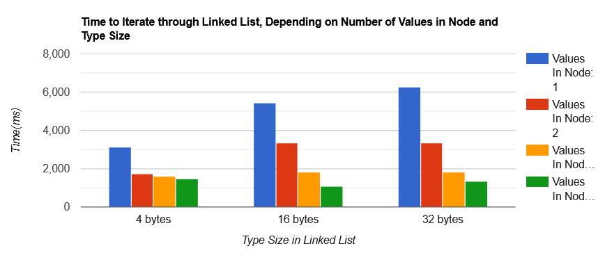
The results look excellent! For smallest type size, iterating through a linked list with two values in node takes 43% less time than iterating through a linked list with one value and this number remains roughly the same for all type sizes.
结果看起来很棒!对于最小的类型大小,遍历具有两个值的节点的链表比遍历具有一个值的节点的链表花费的时间少 43%,并且这个数字对于所有类型大小大致保持不变。
Also note that the bigger the type size in the list, the more sense does it make to have more values in a single linked list node. For 4 bytes type size difference between node with two values and node with four values is small, but for 32 bytes type size this difference is significant.
还要注意,列表中的类型大小越大,在单个链表节点中拥有更多值就越有意义。对于 4 字节类型大小,具有两个值的节点和具有四个值的节点之间的差异很小,但对于 32 字节类型大小,这个差异是显著的。
What about cache performance? What is the number of memory reads7 and data cache miss rate for our test? First lets measure how many memory reads8 does our program make:
缓存性能如何?我们的测试中内存读取次数和数据缓存未命中率是多少?首先让我们测量我们的程序进行了多少次内存读取:
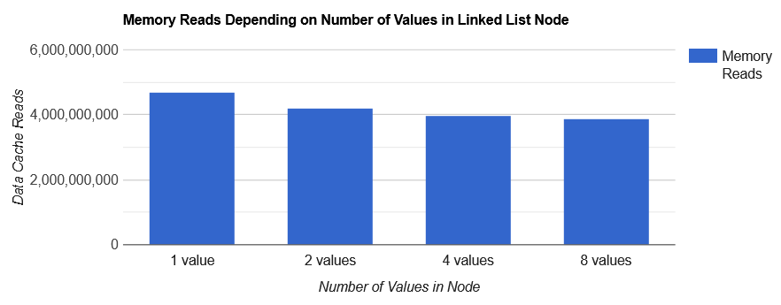
| Values in Node | Memory Reads |
|---|---|
| 1 value | 4,687,587,522 |
| 2 values | 4,218,887,520 |
| 4 values | 3,984,462,522 |
| 8 values | 3,867,275,022 |
As you can see, the more values stored in a single node, there will be less memory reads altogether. This is to be expected since there is less pointer arithmetic involved. Please note that number of memory reads in our case doesn't depend on the type size.
正如你所见,单个节点中存储的值越多,内存读取总数就越少。这是预期的,因为涉及的指针运算更少。请注意,在我们的情况下,内存读取次数不取决于类型大小。
What about cache misses? We used the tool cachegrin\[d to measure cache miss rates9. It can give information about cache misses per function or per line. Here are the results:
缓存未命中呢?我们使用工具 cachegrind 来测量缓存未命中率。它可以提供每个函数或每行的缓存未命中信息。结果如下:
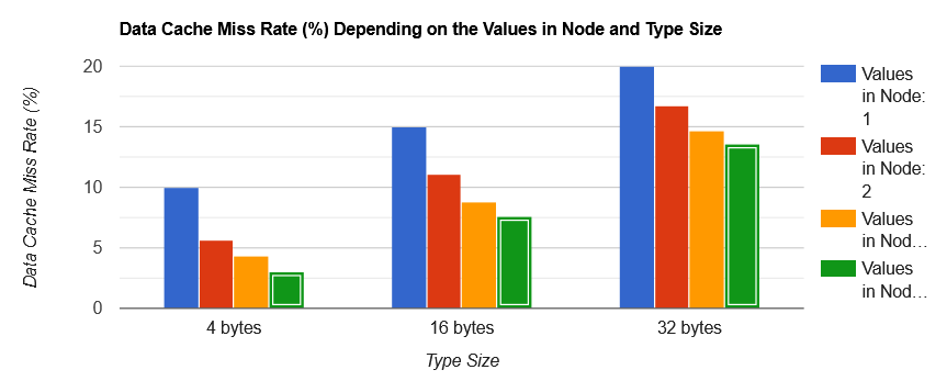
| Type Size | Values in Node: 1 | Values in Node: 2 | Values in Node: 4 | Values in Node: 8 |
|---|---|---|---|---|
| 4 bytes | 10 | 5.6 | 4.4 | 3 |
| 16 bytes | 15 | 11.1 | 8.8 | 7.6 |
| 32 bytes | 20 | 16.7 | 14.7 | 13.6 |
General trend is: if there are more values in a linked list note, there will be less cache misses. For smallest type, cache rate miss is 3% for 8 values in node compared to 10% for 1 value in node. Similar ratio is observed also for larger types.
总体趋势是:如果链表节点中有更多值,缓存未命中就会更少。对于最小的类型,8 个值的节点的缓存未命中率为 3%,而 1 个值的节点为 10%。对于更大的类型也观察到类似的比率。
The other trend: the bigger the type size in a linked list node, the bigger the cache miss rate. For 4 bytes type size cache miss rate is 10% in worst case and 3% in best case. For 32 bytes type size cache miss rate is 20% in worst case and 13.6% in best case. Nothing unexpected. When we are accessing a first value in the node, the cache prefetcher will load values in surrounding memory addresses so when we need them later, they will already be in the cache. If the type is bigger there is less chance that the prefetcher will load useful data, so this is the reason for additional cache misses.
另一个趋势:链表节点中的类型大小越大,缓存未命中率就越高。对于 4 字节类型大小,最坏情况下缓存未命中率为 10%,最好情况下为 3%。对于 32 字节类型大小,最坏情况下缓存未命中率为 20%,最好情况下为 13.6%。这并不意外。当我们访问节点中的第一个值时,缓存预取器将加载周围内存地址中的值,因此当我们稍后需要它们时,它们已经在缓存中。如果类型更大,预取器加载有用数据的机会就更少,这就是额外缓存未命中的原因。
Final Words
So what's the conclusion? There is definitely something interesting to say about data cache optimizations, both in our experiments and generally.
那么结论是什么?无论从本次各项实验来看,还是从通用场景来讲,数据缓存优化都存在不少值得探讨的内容。
Final Words on Experiments
关于实验
So what is the conclusion? Let's talk first about our experiments: all three experiments have shown that careful programming with focus on better using data cache will achieve performance gains. Optimized matrix multiplication has an excellent performance gains compared to the non-optimized version, but apart from matrices, it is rarely the case that we can do a simple manipulation on the data structure to make our structure more cache-friendly. And in my professional experience, I have rarely seen matrices used as data structures.
那么最终结论是什么?我们先来分析本次实验内容:全部 3 组实验均可证明,围绕高效利用数据缓存开展精细化编码能够带来性能提升。经过优化的矩阵乘法相较未优化版本拥有显著的性能增益,但除矩阵以外,极少能仅通过简单修改数据结构就使其适配缓存特性;结合本人项目从业经历,实际工程里也很少选用矩阵作为数据存储结构。
Second experiment was about software prefetching. We indeed see performance increase on binary search with the software prefetching, but performance increase is only relevant for working sets that do not fit the data cache. Please note that software prefetching comes with a price: our system executes more instructions and loads more data into cache which could in some cases lead to worse performance elsewhere10. Good thing about software prefetching is that it is easy to implement and it can be used to speed up iterating through all kinds of structures: linked lists, trees, heaps etc. Yet, careful measurement is needed to make sure that performance gains are worth it.
第二项实验围绕软件预取展开。在二分查找逻辑中启用软件预取后确实观测到性能提升,但这类性能优化仅适用于工作集大小超出数据缓存容量的场景。需要留意,软件预取存在额外开销:系统需要执行更多指令、向缓存载入更多数据,部分场景下还会造成程序其他模块性能下降10。软件预取的优势在于实现成本低,可用于加速链表、树、堆等各类数据结构的遍历操作,但必须经过严谨的性能测算,确认优化收益可以覆盖额外开销。
And our third experiment was about cache friendly linked lists. Again we see with a nice speed improvements. Improvements come from several sources: less memory allocation, smaller data cache miss rate and less instructions needed for pointer arithmetic. The only drawback are more complicated implementation and an increased memory consumption since it might happen that a single node is not optimally filled. But generally, I think these drawbacks are worth the effort.
第三项实验针对缓存友好型链表。该项优化同样实现了可观的运行提速,优化收益来源于三方面:内存申请次数减少、数据缓存缺失率下降、指针运算所需指令量缩减。该方案的不足之处是编码实现复杂度更高,且单个链表节点大概率无法填满存储空间,进而带来内存占用上涨;但综合来看,付出这些开发成本具备实际价值。
Final Words on Data Cache Optimizations
As our experiments have shown, and from my earlier experience, the optimizations indeed bring the performance speeds, and there are numerous applications where this is needed. Performance increase depend on many factors and can range from few percent to 100% or even more.
结合本次实验结果与过往工程经验,缓存优化确实能够提升程序运行速率,大量应用软件场景都有落地该类优化的需求。性能提升幅度受多重条件制约,增幅从百分之几到 100%乃至更高不等。
However, some of the recommendation made here will make your program more difficult to understand and more difficult to debug. And developers have been thought to avoid exactly this, for good reasons. In order to maximally benefit from these optimizations, you will need to carefully profile your program to find the bottlenecks and focus on speeding up those, instead of applying these tips everywhere in your code. Keep your interfaces clean and avoid intermodule dependencies first, then replacing your slow code with a faster one will be simple and you can enjoy the performance increase without sacrificing maintainability.
但本文给出的部分优化方案会提升代码的阅读与调试难度,软件工程领域也一直倡导规避这类设计,背后具备充分的合理性。想要最大化发挥缓存优化的作用,需要借助性能剖析工具定位程序瓶颈,仅针对瓶颈代码落地优化方案,切忌在全量代码中套用优化技巧。优先保证接口简洁、规避模块间冗余依赖,后续替换低效代码时就能以较低成本完成改造,在提升性能的同时不会损害代码可维护性。
notes | 注释
- Modern day multiprocessor systems have complicated hierarchy of cache memories that is beyond the scope of this article
现代多处理器系统拥有架构复杂的高速缓存层级结构,相关内容超出本文论述范围。 - There are also other ways to avoid padding, but this is the simplest.
规避内存对齐填充还有其他实现方案,本方案为最简实现方式。 - It is possible to write directly to memory without going through data cache, e.g. most implementations of memcpy do that. But it is very rare we want to do that in our programs
程序可绕开数据高速缓存直接向内存写入数据,例如绝大多数memcpy的底层实现均采用该方式,但日常开发中极少需要在业务代码里使用该写法。 - Perf is a Linux' profiler, an excellent tool I will write about
Perf是运行在 Linux 平台的性能剖析工具,是一款优质工具,后续我会单独撰文介绍。 - You can execute the tests on your system as well, just download the source code and run
make linked_list_runtimesto execute the tests.
你也可在本机环境运行测试用例,只需下载源码并执行make linked_list_runtimes命令即可启动测试。 - We perform 30 iterations and then measure the average
我们循环执行 30 次运算后统计运算耗时平均值。 - Memory reads and data cache reads are the same thing because all reads go through the cache
内存读操作与数据高速缓存读操作本质等效,所有内存读取请求都会经过高速缓存。 - We measure only memory data reads since iterating through a list doesn't involve memory writes
链表遍历过程不存在内存写入操作,因此我们仅统计内存数据读取次数。 - In our example there were almost no LL cache misses so we measured only L1 cache misses
在本次测试示例中,LL 高速缓存未命中次数趋近于零,因此仅统计 L1 高速缓存未命中数据。 - Example if another program is running on the core that shares the same L1 cache
举例:当其他程序占用共享同一组 L1 高速缓存的处理器核心时。
Use explicit data prefetching to faster process your data structure
利用显式数据预取优化数据结构处理速率
Posted on November 11, 2020
发布于 2020 年 11 月 11 日
Data structure performance is tightly connected to the way they are accessed. And there are two ways to access them: sequentially and randomly. Sequential access is reserved mostly for arrays, and the hardware is really good at it because it can guess what memory location the program is going to access next. But, fast algorithms usually achieve their speed through random accesses, and the hardware cannot do any data prefetching there because it cannot easily guess which memory location will be accessed next. And this leads to poor performance.
数据结构的运行性能和其数据访问方式密切相关,数据访问分为顺序访问与随机访问两类。数组大多采用顺序访问,硬件对该访问模式适配性优异,硬件可预判程序后续要访问的内存地址。但高性能算法大多依托随机访问实现运行提速,硬件无法预判随机访问的目标内存地址,因此无法开展数据预取,最终造成性能下降。
Basic idea
基础原理
If we want to access an element, let's say, in a hash map, we calculate its place in the hash map by applying the hash function, and then we access that element. This is random access. The hardware cannot guess which memory location will be accessed next and therefore cannot prefetch it.
以哈希表的元素访问为例:程序通过哈希函数计算元素在哈希表中的存储位置,随后读取对应元素,该过程属于随机访问。硬件无法预判后续访问地址,也就无法提前预取数据。
If you are lucky enough that the data structure is small and can completely fit the data cache, you should see no slowdowns with random accesses. However, if the size of the data structure is large enough not to fit in the cache (which is typically a few megabytes in size), then we can expect with a large certainty a cache miss for most memory accesses. To illustrate, the work we had to do calculate the hash function of the hash map entry took 20 20 20 cycles, but now the CPU is stuck for 300 300 300 cycles waiting for the piece of data to be fetched from the memory. Can we do better? That depends.
若数据结构体量很小,能够完整存入数据缓存,随机访问不会产生性能损耗。但多数缓存容量仅为数 M B \mathrm{MB} MB,当数据结构超出缓存上限时,绝大多数内存访问都会触发缓存缺失。举例说明:哈希表项的哈希函数计算仅消耗 20 20 20 个时钟周期,CPU 却需要等待 300 300 300 个时钟周期,等候内存完成数据加载。能否优化该问题需要结合实际场景判断。

When accessing a large data structure in a random fashion, the CPU is mostly idle because most accesses to the hash-map entry will result in a cache miss.
以随机方式访问大容量数据结构时,绝大多数哈希表项访问触发缓存缺失,CPU 长期处于空闲等待状态。
If we are accessing a single element, the answer is no. But if we are trying to access several elements, then there is a trick that we can use to speed up things. Here it goes.
单次仅访问一个元素时无法优化;批量访问多个元素时,可借助特定优化手段缩短耗时,具体方案如下。
Modern CPUs offer explicit cache prefetching. What this means is that the program can issue a special prefetch instruction, that will go to the main memory, fetch a cache line and load it into the data cache. All this happens in the background while CPU is free to do other things. When the cache line is fetched, the CPU can access the piece of data quickly.
现代 CPU 支持显式缓存预取功能:程序可调用专用 prefetch 指令,指令会从主内存读取一整条缓存行并存入数据缓存,上述操作在后台异步执行,CPU 可同步执行其他运算;待缓存行加载完毕后,CPU 即可高速读取目标数据。
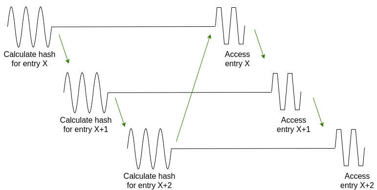
In the case of our hash map, we can split the access to the value into two parts. The first part is calculating the hash function and prefetching the entry. The second part is accessing the entry, doing the comparison, and returning the result.
针对哈希表场景,可将元素读取拆分为两个阶段:第一阶段完成哈希函数运算并预取对应表项;第二阶段读取已预取的表项、完成数据比对并返回运算结果。
Between the first part and the second part, some time needs to pass for the hardware to prefetch the cache line. It is hard (although not impossible) to find a useful thing to do during this short time if we are processing a single element.
硬件需要一定时长完成缓存行预取,因此两个执行阶段之间需要预留间隔。若仅处理单个元素,很难在预取等待间隙填充有效运算。
But if we are processing a batch of elements, we can do the following: iterate through the batch, do the prefetching part for element X X X, and while the value is prefetched, go and do other operations for other elements. What this other operation is, that depends on how we write your algorithm.
批量处理元素时可采用如下思路:遍历整批数据,对第 X X X 个元素发起预取请求;在等待该元素预取完成的间隙,执行其余元素的相关运算,补充运算内容由算法逻辑决定。
Nano threads
微线程预取方案
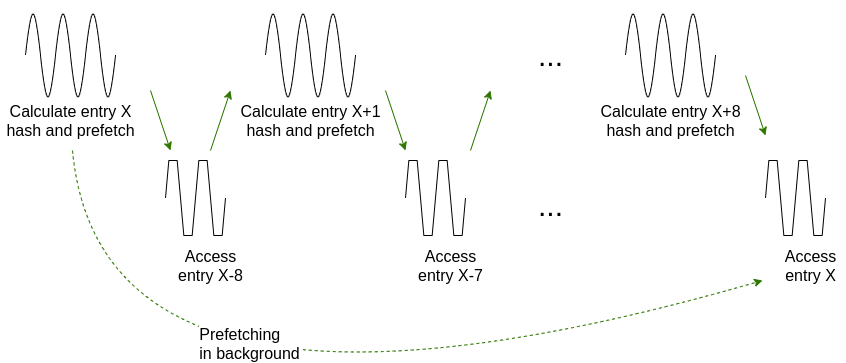
One way to organize the prefetch/access split is nano threads. The idea is to pick a constant, for example, 16 16 16. Then we do 16 16 16 prefetches for elements N , N + 1 , ... , N + 15 N, N+1, \dots, N+15 N,N+1,...,N+15 followed by 16 16 16 accesses for the same elements in the same order.
微线程是拆分预取与访问流程的实现方案之一:选定一个固定数值(例如 16 16 16),先对 N 、 N + 1 、 ... 、 N + 15 N、N+1、\dots、N+15 N、N+1、...、N+15 共 16 16 16 个元素批量发起预取,预取全部结束后,再按相同顺序依次访问上述 16 16 16 个元素。
Nano threads: we first perform prefetches, then we perform accesses
微线程机制:先批量执行预取操作,再统一执行数据访问。
It is important to pick the constant properly. Too small, and the access phase will start before the hardware completes the prefetching. Too large, and some of the prefetched values will be evicted from cache.
固定参数的取值需要合理把控:参数过小会导致预取尚未完成就提前进入访问阶段;参数过大则部分已预取数据会被缓存淘汰。
The approach is called nano-threads because it resembles instantiating a bunch of threads that all do the same job. Please note that no actual threading is involved, the program runs completely serially.
该方案命名为微线程,是因为运行逻辑和多线程批量处理任务类似,但实现过程不启用操作系统线程,程序全程串行执行。
Alternating prefetch/access
交替预取访问方案
I named the second approach alternating prefetch/access because it does exactly that, it alternates between prefetching for element X X X and accessing for already prefetched element X − n X-n X−n.
第二种优化方案命名为交替预取访问,方案核心逻辑为交替执行两项操作:对第 X X X 个元素发起预取、访问已完成预取的第 X − n X-n X−n 个元素。
In the alternating prefetch/access approach, the program alternates between prefetching for element X X X and accessing prefetched element X -- n X -- n X--n
交替预取访问机制:程序交替执行 X X X 元素预取、 X − n X-n X−n 已预取元素读取。
Again it is important to pick the constant n n n properly for the same reason as with the previous approach.
和微线程方案一致,参数 n n n 需要合理选取,避免预取未完成或缓存数据被淘汰。
Which approach is better?
两种方案优劣对比
There is no clear answer. From the performance perspective, they are similar. From the simplicity point of view, that again depends on the underlying data structure. In our hash map example, the alternating prefetch/access approach was simpler and also faster, but this doesn't necessarily have to be the case with other data structures.
两种方案没有绝对优劣之分:运行性能层面二者表现相近;实现复杂度由底层数据结构决定。在本文哈希表测试场景中,交替预取访问实现更简易、性能更优,但该结论不适用于全部数据结构。
For both approaches, we need to experimentally determine the value of the constant. A good rule of thumb is to start with constant 16 16 16, and then go up or down until reaching the best performance. Also note, that the constant that works best on one system might not be the same that works on another. In that case you might want to perform the calibration in runtime.
两类方案的参数都需要通过实测确定,常规调试思路:初始参数设为 16 16 16,上下微调参数直至性能最优。最优参数存在硬件平台差异性,跨设备运行时可在程序运行阶段动态校准参数。
What other people already did?
现有同类落地实践
Well, this idea is not new and has been tried out and found working. In a talk by G. Nishanov [Nano-coroutines to the Rescue! (Using Coroutines TS, of Course) , the author first presents a simple binary search algorithm and then goes into details on how to transform this algorithm by applying the principles we already discussed.
预取拆分优化并非全新思路,已有落地案例验证优化有效性。G. Nishanov 在《微型协程实战(基于协程 TS 标准)》分享中,以基础二分查找算法为例,详述如何依托前文预取思路改造原有算法。
Given an element to find in a sorted array of size N N N, it will take approximately log 2 ( N ) \log_2(N) log2(N) steps to check if the element is in the array. Most of the checks will result in a cache miss. So the idea is to split each check into two phases: a prefetch phase and an access phase. And the program is alternating between prefetching element X X X and accessing already prefetched element Y Y Y.
在长度为 N N N 的有序数组中查找目标元素,需要约 log 2 ( N ) \log_2(N) log2(N) 次比对,绝大多数比对操作会触发缓存缺失。优化思路:将单次查找拆分为预取阶段与访问阶段,程序交替执行 X X X 元素预取、 Y Y Y 元素(已预取)访问。
The author shows how it is done simply with coroutines, and I suggest you watch because the concept of coroutines is fun to know and useful in this context, albeit not necessary. The resulting speed-up is what interests us: if the sorted array cannot fit the last-level cache (which is typically a few megabytes), it takes 26 n s 26\ \mathrm{ns} 26 ns per lookup. However, when the author used batch processing with prefetch it is 10 n s 10\ \mathrm{ns} 10 ns per lookup. Not bad.
作者依托协程完成优化落地,协程知识可拓展开发思路,推荐观看分享视频;优化效果是本次关注重点:有序数组超出末级缓存(常规容量数 M B \mathrm{MB} MB)时,原始单次查找耗时 26 n s 26\ \mathrm{ns} 26 ns,引入批量预取优化后单次查找缩短至 10 n s 10\ \mathrm{ns} 10 ns,优化收益可观。
Our experiment
自研对照实验
To try this out, we made our own experiment. We created a hash map called fast_hash_map that implements methods:
为验证优化效果,本文搭建自研实验,实现 fast_hash_map 哈希表结构,包含三类接口:
-
find_multiple_simple checks if
std::vectorof inputs is present in the hash map, without any prefetchingfind_multiple_simple:无预取逻辑,校验输入std::vector内元素是否存在于哈希表 -
find_multiple_nanothreads checks if
std::vectorof inputs is present in the hash map, using prefetch with nano threads implementationfind_multiple_nanothreads:基于微线程预取,校验输入std::vector内元素是否存在于哈希表 -
find_multiple_alternate checks if
std::vectorof inputs is present in the hash map, using prefetch with alternate prefetch/access approachfind_multiple_alternate:基于交替预取访问,校验输入std::vector内元素是否存在于哈希表
There was a question on how to deal with collisions in our hash map. A hash map entry can have zero (entry is available), one (entry is occupied), or more than one element (there are collisions with the entry). Many collisions slow down the access to the hash map, but with a good hash function and rehashing when the hash map becomes too big, typically there shouldn't be many collisions.
实验同步考量哈希冲突处理逻辑:哈希表表项分为三种状态:空项(无数据)、单元素项(已占用)、多元素项(存在哈希冲突)。大量冲突会拖慢哈希表访问效率,选用优质哈希函数并在装填率过高时执行重哈希,可大幅减少冲突频次。
Hash maps are typically implemented using an array. A simple implementation is a data structure where each element of the array is a pointer to another array with one or more elements. This implementation has one major drawback when it comes to cache efficiency: to get to the first value in the entry, the program needs to follow two pointers, which often results in two cache misses!
哈希表底层普遍依托数组实现。简易实现方案中,主数组每个成员存储子数组指针,子数组存放实际数据;该方案缓存短板突出:读取表项首个数据需要两次指针寻址,极易触发两次缓存缺失。
Simple implementation of hash map. If the entry is occupied, we will need to follow two pointers. The first is to get the entry in the hash map array. If the count of the entry > 0 > 0 >0, then we need to follow the second pointer. Following two pointer typically results in two cache misses.
哈希表简易实现结构:表项被占用时需要两次指针寻址,首次寻址定位主数组表项,若表项数据数量 > 0 > 0 >0,则二次寻址指向数据子数组,两次寻址大概率触发两次缓存缺失。
Another, more complicated implementation, stores the first element of the hash map inside the entry itself, and the pointers to other elements in an additional array with one or more elements. The good thing about this approach is that in the typical case (zero or one value in the entry) we will have only one cache miss. In case of collisions, we will have two cache misses.
进阶实现方案:首个数据直接存储在主数组表项内部,冲突产生的多余数据存入额外子数组。常规场景(空项或单数据项)仅触发一次缓存缺失,仅出现哈希冲突时才会产生两次缓存缺失。
Advanced hash map implementation. We use the additional array only to store collisions. In case of no collisions, this means one cache miss and better speed.
哈希表进阶实现结构:额外子数组仅用于存放冲突数据,无冲突场景仅单次缓存缺失,访问效率更高。
The input is given as a vector of values and the result is returned as a vector of bools. So how did it measure up?
实验输入为数值数组,输出为布尔结果数组,各方案实测数据如下。
We used a hash map with N N N entries. First we insert 0.7 ⋅ N 0.7 \cdot N 0.7⋅N entries into it, and then we remove 0.3 ⋅ N 0.3 \cdot N 0.3⋅N entries from it. So the hash map is halfway full.
测试哈希表总表项数为 N N N,先插入 0.7 × N 0.7 \times N 0.7×N 组数据,再删除 0.3 × N 0.3 \times N 0.3×N 组数据,最终哈希表装填率约 50 % 50\% 50%。
Let's see how the three implementations (STL, simple and advanced) measure against each other when no prefetching is involved.
首先对比无预取逻辑下,STL 标准哈希表、简易哈希表、进阶哈希表三者的耗时表现。
| No of entries and iterations 条目数量与迭代次数 | STL std::unordered_set STL 标准无序集合 | simple hash map 简易哈希表 | advanced hash map 进阶哈希表 |
|---|---|---|---|
| 32 entries 2M iterations 32 个条目、 2 × 10 6 2 \times 10^6 2×10⁶ 次迭代 | 1435 m s 1435\ \mathrm{ms} 1435 ms | 1824 m s 1824\ \mathrm{ms} 1824 ms | 1427 m s 1427\ \mathrm{ms} 1427 ms |
| 1M entries 64 iterations 1 × 10 6 1 \times 10^6 1×10⁶ 个条目、 64 64 64 次迭代 | 2849 m s 2849\ \mathrm{ms} 2849 ms | 4161 m s 4161\ \mathrm{ms} 4161 ms | 2481 m s 2481\ \mathrm{ms} 2481 ms |
| 64M entries 1 iteration 64 × 10 6 64 \times 10^6 64×106 个条目、 1 1 1 次迭代 | 5853 m s 5853\ \mathrm{ms} 5853 ms | 5838 m s 5838\ \mathrm{ms} 5838 ms | 3785 m s 3785\ \mathrm{ms} 3785 ms |
Hash map comparisons for a simple case without prefetching
无预取时三类哈希表性能对照
For small to medium loads, the STL implementation looks good which is reasonable to expect. STL is used for general-purpose programming, it will be used by millions of developers, and mostly on small to medium loads.
中小数据量场景中 STL 哈希表性能表现优异,符合设计定位:STL 面向通用开发场景,海量开发者多用于中小体量数据处理。
For large loads ( 64 64 64 million entries), the advanced hash map is the best. It is 35 % 35\% 35% faster than both STL and simple hash map implementation. This example sheds light on the importance of memory layout! By decreasing the number of pointer dereferencing from two to one, we achieve a large speedup. This is applicable for all data structures, not just here. A B* tree is much faster than the red-black tree for the same reason: B* tree keeps more than one value in the node; it better uses cache lines and it is shallower. Too bad that in C++, all std::map and std::set are implemented using red-black trees "for historical reasons".
6400 6400 6400 万条目的大数据场景下进阶哈希表性能最优,相比 STL 与简易哈希表提速约 35 % 35\% 35%。该数据直观体现内存排布设计的作用:指针寻址次数由两次缩减至一次即可实现显著提速,该优化逻辑适用于全品类数据结构。B* 树节点存储多组数据、缓存利用率更高且树深度更小,因此运行速率优于红黑树;受历史实现因素影响,C++ 的 std::map、std::set 底层均采用红黑树实现。
Now, let's see what happens when the prefetching comes into play. Here are the results for the large load:
引入预取优化后,大数据量场景实测数据如下:
| Hash map implementation 哈希表类型 | No prefetching 无预取 | Nano-threads approach 微线程预取 | Alternating prefetch/access approach 交替预取访问 |
|---|---|---|---|
| STL std::unordered_set STL 标准无序集合 | 5853 m s 5853\ \mathrm{ms} 5853 ms | -- | -- |
| Simple hash map 简易哈希表 | 5838 m s 5838\ \mathrm{ms} 5838 ms | 3522 m s 3522\ \mathrm{ms} 3522 ms | 3356 m s 3356\ \mathrm{ms} 3356 ms |
| Advanced hash map 进阶哈希表 | 3785 m s 3785\ \mathrm{ms} 3785 ms | 2257 m s 2257\ \mathrm{ms} 2257 ms | 2009 m s 2009\ \mathrm{ms} 2009 ms |
Comparison of prefetching on a large load ( 64 64 64 million entries), with and without prefetching
6400 6400 6400 万条目大数据量:有无预取方案性能对照
We went from 5.8 5.8 5.8 seconds on the regular STL implementation, to 2 2 2 seconds with the advanced hash map with prefetching. A very good result. But this is the large load. What happens to small and medium loads?
原始 STL 方案耗时 5853 m s 5853\ \mathrm{ms} 5853 ms,搭配预取的进阶哈希表耗时降至 2009 m s 2009\ \mathrm{ms} 2009 ms,优化幅度突出。接下来测试小、中数据量场景的预取优化效果。
| Hash map implementation 哈希表类型 | No prefetching 无预取 | Nano-threads approach 微线程预取 | Alternating prefetch/access approach 交替预取访问 |
|---|---|---|---|
| STL std::unordered_set STL 标准无序集合 | 1435 m s 1435\ \mathrm{ms} 1435 ms | -- | -- |
| Simple hash map 简易哈希表 | 1824 m s 1824\ \mathrm{ms} 1824 ms | 1910 m s 1910\ \mathrm{ms} 1910 ms | 2376 m s 2376\ \mathrm{ms} 2376 ms |
| Advanced hash map 进阶哈希表 | 1427 m s 1427\ \mathrm{ms} 1427 ms | 1514 m s 1514\ \mathrm{ms} 1514 ms | 2015 m s 2015\ \mathrm{ms} 2015 ms |
Comparison of prefetching on a small load ( 32 32 32 entries, 2 M 2\mathrm{M} 2M iterations), with and without prefetching
32 32 32 条目、 2 × 10 6 2 \times 10^6 2×10⁶ 迭代小数据量:有无预取方案性能对照
Measuring small loads is always difficult. The batch processing algorithms need to allocate memory from the system (to store the results) and this can influence the measurement results. But we tried to make all algorithms do the same thing for the sake of measurements. We know that from one of the previous posts that prefetch instruction actually slows down the program in case the data is already in the data cache (which is the case for small load). So, this optimization is actually a slow down on a small load.
小数据量场景测试存在干扰因素:批量运算需要申请系统内存存储结果,会轻微干扰计时。实验已统一各方案内存操作逻辑;结合往期文章结论可知:小数据场景数据全部驻留缓存,额外执行预取指令会引入指令开销,反而拖慢程序运行。
| Hash map implementation 哈希表类型 | No prefetching 无预取 | Nano-threads approach 微线程预取 | Alternating prefetch/access approach 交替预取访问 |
|---|---|---|---|
| STL std::unordered_set STL 标准无序集合 | 2849 m s 2849\ \mathrm{ms} 2849 ms | -- | -- |
| Simple hash map 简易哈希表 | 4161 m s 4161\ \mathrm{ms} 4161 ms | 2409 m s 2409\ \mathrm{ms} 2409 ms | 2481 m s 2481\ \mathrm{ms} 2481 ms |
| Advanced hash map 进阶哈希表 | 3184 m s 3184\ \mathrm{ms} 3184 ms | 1731 m s 1731\ \mathrm{ms} 1731 ms | 1854 m s 1854\ \mathrm{ms} 1854 ms |
Comparison of prefetching on a medium load ( 1 M 1\mathrm{M} 1M entries, 64 64 64 iterations), with and without prefetching
1 × 10 6 1 \times 10^6 1×10⁶ 条目、 64 64 64 次迭代中数据量:有无预取方案性能对照
For medium load, the prefetching makes sense. It is not as fast as in the case of a large load, but the numbers are better than with no prefetching.
中等数据量场景预取优化收益有效,优化幅度不及大数据场景,但各项指标均优于无预取实现。
As you might have seen, as the load becomes larger and larger, so prefetching makes more and more sense.
综上可得:数据体量越大,显式预取的优化收益越显著。
Final Words
总结
This is not a technique that you will see every day and that is meant for everyday use. But in case performance is important and the load is large, this technique can achieve great results with a little effort. Keeping the CPU when it needs to wait for data from the memory is an important way to speed up your program.
显式预取不属于通用常规优化手段,但对性能敏感、大数据量的业务场景,少量开发改造即可收获可观提速。消除 CPU 等待内存数据的空闲空档,是程序性能优化的有效思路。
突破计算机性能瓶颈的利器:CPU Cache
原创 小牛呼噜噜|2023 年 7 月 12 日 20:07|江苏
本文围绕计算机存储器分支之一的 CPU 高速缓冲存储器开展论述,该器件简称 CPU Cache \boldsymbol{\text{CPU Cache}} CPU Cache。
缓存为计算机工程领域通用专业名词,应用场景不局限于 CPU 硬件架构,例如 CDN \text{CDN} CDN 可实现站点资源缓存、浏览器可缓存页面图像与流媒体数据。本文限定讨论范围为狭义硬件缓存,即 CPU Cache \texttt{CPU Cache} CPU Cache,正文统一简写为缓存或 Cache \text{Cache} Cache。
1 计算机性能的瓶颈
在冯·诺依曼体系架构下,计算机存储器件采用分层排布结构,整体排布呈金字塔层级,自上而下依次为通用寄存器、高速缓存、主存储器(内存)、机械存储设备等。
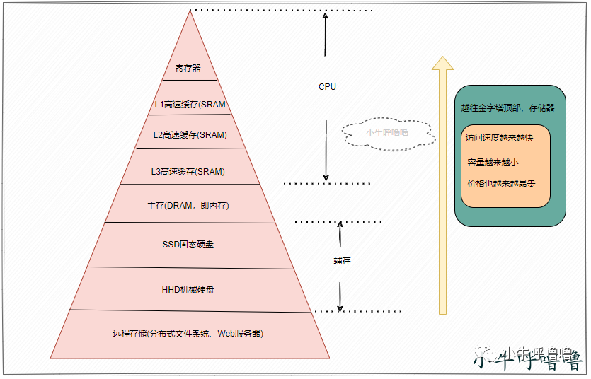
存储器件与 CPU \text{CPU} CPU 的物理距离和器件参数存在对应规律:器件距离 CPU \text{CPU} CPU 越近,数据访问时延越低、存储容量越小、单位字节硬件制造成本越高。
以标称主频 3.0 GHz 3.0\ \text{GHz} 3.0 GHz 的 CPU \text{CPU} CPU 为例:通用寄存器的数据访问可在 1 1 1 个时钟周期内完成,单时钟周期作为 CPU \text{CPU} CPU 时序基准单位,对应时长约 0.3 ns 0.3\ \text{ns} 0.3 ns;主存单次数据访问耗时约 120 ns 120\ \text{ns} 120 ns;固态硬盘单次访问耗时区间为 50 ∼ 150 μ s 50 \sim 150\ \mu\text{s} 50∼150 μs;机械硬盘单次访问耗时区间为 1 ∼ 10 ms 1 \sim 10\ \text{ms} 1∼10 ms;跨网络的数据访问耗时可达数十毫秒。
为量化不同存储层级的时延差距,建立时序缩放模型:设定单时钟周期等效现实时长 1 s 1\ \text{s} 1 s,则寄存器访问耗时等效 1 s 1\ \text{s} 1 s,主存访问等效 6 min 6\ \text{min} 6 min,固态硬盘访问等效 2 ∼ 6 d 2 \sim 6\ \text{d} 2∼6 d,机械硬盘访问等效 1 ∼ 12 mon 1 \sim 12\ \text{mon} 1∼12 mon,网络数据访问等效数年时长。由缩放模型可见, CPU \text{CPU} CPU 运算速率与大容量存储器件的数据读取速率分属不同数量级。
电子计算机发展早期的硬件架构未集成 CPU Cache \text{CPU Cache} CPU Cache,该阶段 CPU \text{CPU} CPU 工作主频偏低,运算速率不优于同期主存读写速率, CPU \text{CPU} CPU 对指令与数据的读写操作直接面向主存完成。
自 1980 1980 1980 年代硬件工艺迭代后, CPU \text{CPU} CPU 主频提升速率持续领先主存性能迭代速率,二者读写时延差值持续扩大;在冯·诺依曼架构约束下, CPU \text{CPU} CPU 访问主存的读写时延成为整机数据吞吐的制约条件。
DRAM \text{DRAM} DRAM 即动态随机存取存储器,为主存核心存储颗粒;图片来源:How L1 and L2 CPU Caches Work, and Why They're an Essential Part of Modern Chips
为抵消 CPU \text{CPU} CPU 与主存之间的速率差值、缩短主存访问耗时,硬件体系引入 CPU Cache \texttt{CPU Cache} CPU Cache。缓存的数据访问速率仅次于通用寄存器,在硬件链路中承担 CPU \text{CPU} CPU 与主存之间的数据中转功能。
2 缓存及其发展历史
CPU Cache \texttt{CPU Cache} CPU Cache 基于 SRAM \boldsymbol{\text{SRAM}} SRAM(Static Random-Access Memory,静态随机存储器)芯片实现,该类器件通电状态下可稳定留存存储数据,断电后内部数据全部丢失。
现行商用 CPU \text{CPU} CPU 的片上缓存分为三级独立存储单元,依次命名为 L1 Cache \boldsymbol{\text{L1 Cache}} L1 Cache、 L2 Cache \boldsymbol{\text{L2 Cache}} L2 Cache、 L3 Cache \boldsymbol{\text{L3 Cache}} L3 Cache。
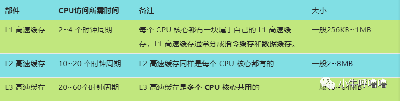
缓存单元排布满足固定规律:存储单元距离 CPU \text{CPU} CPU 核心越近,数据访问时延越低、标称容量越小、单片硬件制造成本越高,缓存层级典型物理分布结构参考下图。
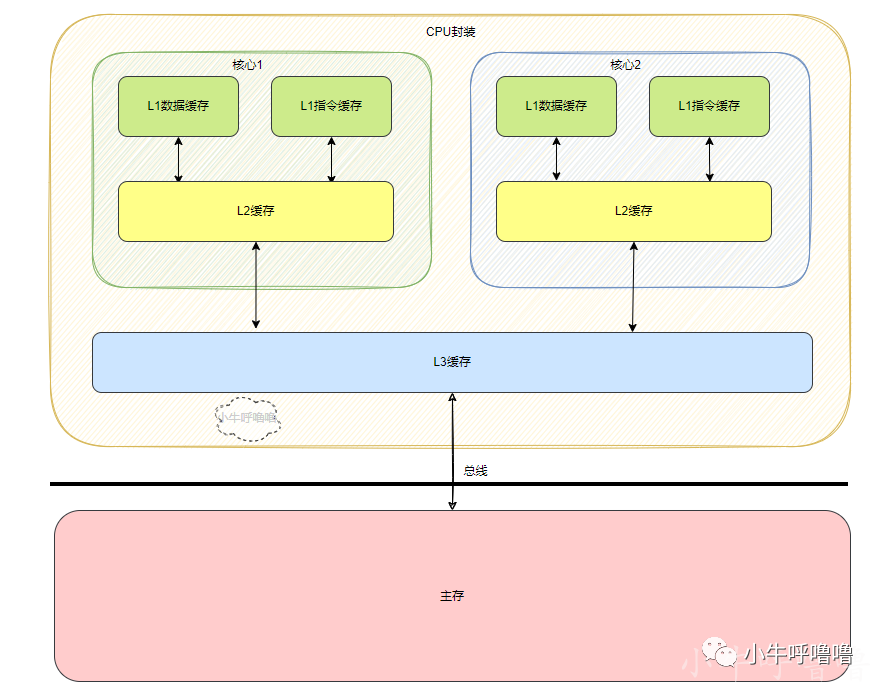
以 Intel 系列处理器为研究样本梳理 Cache \text{Cache} Cache 迭代历程:
-
80286 及更早处理器
该代产品硬件架构未配置片上缓存, CPU \text{CPU} CPU 主频参数低于同期主存读写速率,处理器所有读写指令直接寻址主存。
-
80386 处理器
该代产品量产阶段, CPU \text{CPU} CPU 与主存的速率失配问题逐步显现,低速主存限制处理器运算性能释放。Intel 通过主板拓展接口增设 外部 Cache \texttt{外部 Cache} 外部 Cache,依托外置缓存器件优化 80386 的整机数据吞吐效率。
-
80486 处理器
处理器片内集成容量 8 KB 8\ \text{KB} 8 KB 的 L1 Cache \texttt{L1 Cache} L1 Cache,同时保留主板拓展接口以搭载外置 L2 Cache \text{L2 Cache} L2 Cache,外置缓存容量区间为 128 KB ∼ 256 KB 128\ \text{KB} \sim 256\ \text{KB} 128 KB∼256 KB;该阶段 L1 Cache \text{L1 Cache} L1 Cache 未做指令、数据分区设计。
该代产品配置的 8 KB L1 Cache 8\ \text{KB}\ \text{L1 Cache} 8 KB L1 Cache 可匹配同期处理器的访存需求,缓存命中率与一、二级缓存容量的关联特性参考下图。
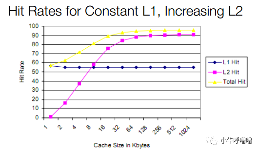
图片来源:How L1 and L2 CPU Caches Work, and Why They're an Essential Part of Modern Chips
由命中率变化曲线可得:单纯扩容 L1 Cache \texttt{L1 Cache} L1 Cache 无法实现缓存命中率的明显提升,同时推高硬件生产成本,投入产出比偏低; L2 Cache \texttt{L2 Cache} L2 Cache 容量扩容可推动整体缓存命中率快速上涨,大容量、低成本、访问时延略高的二级缓存成为硬件优化的优选路径。
- Pentium‑1(80586)系列处理器
产品采用超标量双流水线架构,集成两路并行整数运算流水线,需要同步完成指令读取与数据存取操作。硬件将单片 L1 Cache \texttt{L1 Cache} L1 Cache 拆分为独立指令缓存与数据缓存,两类子缓存标称容量均为 8 KB 8\ \text{KB} 8 KB;该时期 L2 Cache \texttt{L2 Cache} L2 Cache 仍挂载于主板拓展插槽。后续 Pentium Pro(80686)处理器完成架构优化, L2 Cache \texttt{L2 Cache} L2 Cache 正式集成至处理器芯片内部。
- 多核架构迭代阶段
Pentium D、Pentium EE 多核处理器中,各运算核心配置独立的 L1 Cache \texttt{L1 Cache} L1 Cache 与 L2 Cache \texttt{L2 Cache} L2 Cache,核心间缓存数据同步依托前端总线完成。Core Duo(酷睿)系列落地 Smart cache \text{Smart cache} Smart cache 共享缓存方案, L2 Cache \texttt{L2 Cache} L2 Cache 变更为多核共用存储资源,该方案奠定现代处理器缓存的基础架构规范。
当前主流处理器沿用三级缓存架构,即 L1 Cache \texttt{L1 Cache} L1 Cache、 L2 Cache \texttt{L2 Cache} L2 Cache、 L3 Cache \texttt{L3 Cache} L3 Cache; L1 \text{L1} L1、 L2 \text{L2} L2 缓存隶属于单个运算核心, L3 \text{L3} L3 缓存由处理器内部全部核心共享。部分新型处理器已搭载 L4 Cache \text{L4 Cache} L4 Cache,后续硬件迭代中缓存分级类型存在继续拓展的可能。
3 缓存弥补 CPU 与内存性能差异的实现原理
缓存优化整机访存效率的理论依托为局部性原理 。缓存存取速率仅次于片上寄存器, CPU \text{CPU} CPU 与主存的性能落差来源于二者读写时延的数量级差距;硬件通过提高缓存的访存占比、削减 CPU \text{CPU} CPU 直接寻址主存的频次,实现整机数据吞吐能力提升。
局部性原理划分为 时间局部性 \texttt{时间局部性} 时间局部性 与 空间局部性 \texttt{空间局部性} 空间局部性 两类约束规则:
- 时间局部性:已完成一次寻址的存储地址,在短周期时序内存在重复寻址概率,循环代码段为该规律的典型应用场景。
- 空间局部性:某一存储地址触发寻址操作后,该地址相邻的连续存储单元在后续时序中具备较高寻址概率。
缓存的硬件调度逻辑依照局部性原理设计:
- 硬件临时存储 CPU \text{CPU} CPU 近期从主存读取的指令与数据,依托时间局部性,该部分内容在短时间窗口内存在重复调用需求;
- 处理器从主存读取目标数据时,同步加载目标地址周边连续存储单元的数据并写入缓存,依托空间局部性,相邻存储区域的数据存在后续访问可能。
CPU \text{CPU} CPU 执行访存指令时遵循分级检索顺序:优先检索 L1 Cache \texttt{L1 Cache} L1 Cache,命中数据则直接从缓存读取;未命中时逐级检索 L2 Cache \texttt{L2 Cache} L2 Cache、 L3 Cache \texttt{L3 Cache} L3 Cache;全部缓存检索失效后,处理器发起主存寻址请求。
4 尾语
本文依次阐述计算机访存瓶颈的形成诱因、 CPU Cache \text{CPU Cache} CPU Cache 的硬件迭代历程、缓存优化访存速率的底层原理。后续内容将继续展开 Cache \text{Cache} Cache 硬件组织结构、缓存一致性协议、程序层面依托缓存特性优化代码运行效率等内容。
参考资料
- https://www.extremetech.com/extreme/188776-how-l1-and-l2-cpu-caches-work-and-why-theyre-an-essential-part-of-modern-chips
- http://www.cpu-zone.com/80486.htm
CPU Cache 是如何映射与寻址的?
原创|小牛呼噜噜|2023 年 8 月 29 日 19:15|江苏
本文承接上文内容,围绕 CPU Cache \texttt{CPU Cache} CPU Cache 的硬件组织结构、主存--缓存地址映射规则与硬件寻址逻辑展开论述。
1 CPU Cache 的组织结构
CPU Cache \texttt{CPU Cache} CPU Cache 在硬件层面划分为多级分组结构:整体划分为若干个 Set \texttt{Set} Set(缓存组),单个 Set \texttt{Set} Set 内部包含多条独立 Cache Line \texttt{Cache Line} Cache Line(缓存行)。 Cache Line \texttt{Cache Line} Cache Line 为缓存硬件的最小存取单元,工程领域亦记作 Block \texttt{Block} Block(存储块);处理器对缓存的数据读写操作以整行作为基本粒度,不支持单字节独立存取。
主流商用处理器的 Cache Line \texttt{Cache Line} Cache Line 标准容量为 64 Byte \boldsymbol{64\ \text{Byte}} 64 Byte,硬件设计可选用其他规格容量。缓存块容量与缓存命中率存在连续变化规律:块容量取值偏小时,缓存命中率处于低位;随块容量逐步增大,空间局部性规律生效,命中率快速抬升。
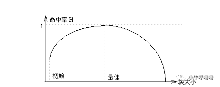
命中率在某一最优块容量处到达峰值;超出最优值后,继续扩容缓存块将造成命中率缓慢下降。该变化由两项约束条件决定:块容量过大时,单次载入缓存的冗余数据占比上升,大量数据在生命周期内不会被处理器访问;同时块尺寸持续扩大会弱化时间局部性带来的访问增益。
单条 Cache Line \texttt{Cache Line} Cache Line 由三类字段构成: Valid \texttt{Valid} Valid(有效标志位)、 Tag \texttt{Tag} Tag(地址标记)、 Data \texttt{Data} Data(数据域),各字段功能定义如下:
- Data \texttt{Data} Data:用于连续存放一段主存地址对应的原始数据;
- Tag \texttt{Tag} Tag:存储当前数据段对应的高位地址标识,作为缓存匹配检索依据;
- Valid \texttt{Valid} Valid:标记本行缓存数据的有效性,辅助硬件完成命中判别。
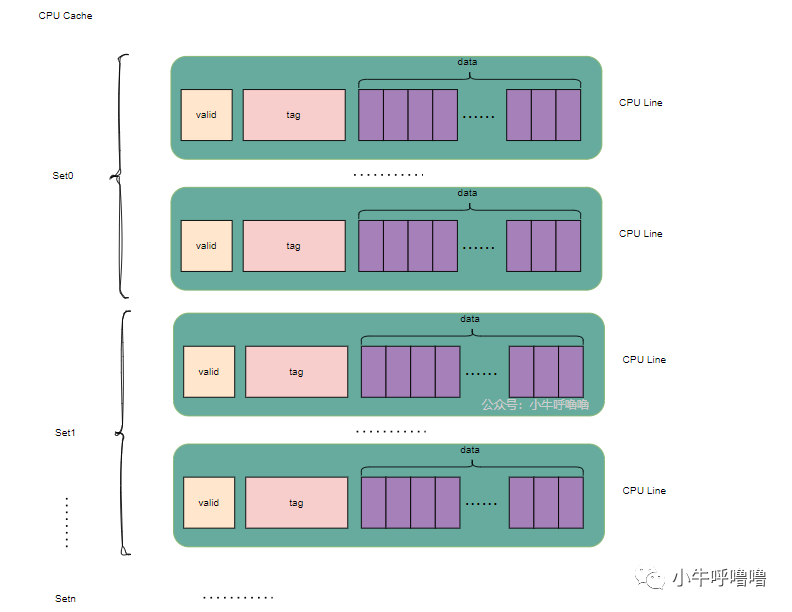
2 Cache 与主存地址映射
Cache \text{Cache} Cache 的单字节制造成本高于主存、硬件总容量远小于主存,但需要完整承接主存的数据缓存需求。受容量约束限制,主存存储块无法与缓存行实现一一绑定,因此需要标准化的地址映射规则,建立主存地址至缓存物理位置的对应关系。
现行硬件架构包含三类成熟映射方案:直接映射、全相联映射、组相联映射。
- 直接映射:单个 Set \texttt{Set} Set 仅配置一条 Cache Line \texttt{Cache Line} Cache Line,组索引确定后无需组内多标记比对;
- 全相联映射:全局仅配置单个 Set \texttt{Set} Set,全部缓存行统一归入该缓存组;
- 组相联映射:配置多组 Set \texttt{Set} Set,单组内部包含多条缓存行;工程中以**路( Way \text{Way} Way)**描述单组缓存行数量,例如 6 6 6 路组相联代表单个 Set \texttt{Set} Set 内置 6 6 6 条独立 Cache Line \texttt{Cache Line} Cache Line。
2.1 直接映射
直接映射在主存块与缓存行之间建立静态绑定规则,任意主存存储块仅能映射至缓存内唯一指定缓存行。
补充说明:Linux 内核文件系统加速模块早期采用块缓存机制,区别于现代基于页管理的页缓存实现方案。
以主存划分为 8 8 8 个存储块、缓存配置 4 4 4 条缓存行为示例:
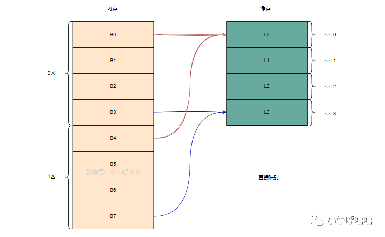
示例中主存块 B0、B4 \text{B0、B4} B0、B4 固定映射至缓存第 0 0 0 行,主存块 B3、B7 \text{B3、B7} B3、B7 固定映射至缓存第 3 3 3 行,其余存储块遵循同类约束。
映射计算公式:主存块编号对缓存总行数做取模运算,运算结果即为目标缓存行序号。该规则等价于按照缓存总容量对主存地址空间做均等分区。
方案特性:
- 优势:硬件译码逻辑简单、检索时延低、地址转换硬件开销小;
- 短板:固定映射规则造成存储空间利用率受限,空闲缓存行无法接纳冲突数据,块冲突发生概率偏高;冲突频发时主存数据反复替换同一缓存行,拉低整体命中率。
该架构多用于大容量片上缓存场景。
2.2 全相联映射
全相联映射无分组约束,任意主存存储块可载入缓存内任意空闲缓存行。
方案特性:
- 优势:空间利用率高、存储块冲突概率低,仅在全部缓存行填满后才出现数据替换;
- 短板:单次访存需要并行比对全部缓存行的 Tag \texttt{Tag} Tag 字段,硬件比较电路规模大、访问延迟偏高。
该架构多用于小容量专用缓存。
2.3 组相联映射
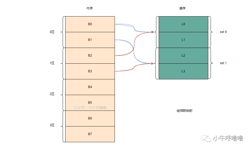
组相联映射为前两类方案的折中实现,规则概括为:组间遵循直接映射、组内遵循全相联映射。主存块所属缓存组由地址译码唯一确定,数据在目标缓存组内部可自由选用任意空闲缓存行。
寻址流程优化:硬件先通过组索引锁定目标缓存组,仅在组内有限条数缓存行中完成 Tag \texttt{Tag} Tag 比对。该设计兼顾冲突概率与访问时延,为当代通用处理器的主流缓存实现方案。
3 Cache 寻址方式
以 Intel 通用处理器典型 L1 Cache \text{L1 Cache} L1 Cache 参数作为算例: 32 KB \boldsymbol{32\ \text{KB}} 32 KB 容量、 8 8 8 路组相联架构、 Cache Line = 64 Byte \texttt{Cache Line}=64\ \text{Byte} Cache Line=64 Byte。
单路缓存总行数 = 32 KB 64 Byte ÷ 8 = 64 单组寻址空间 = 64 × 64 Byte = 4096 Byte = 4 KB \begin{align*} \text{单路缓存总行数} &= \frac{32\ \text{KB}}{64\ \text{Byte}} \div 8 = 64 \\ \text{单组寻址空间} &= 64 \times 64\ \text{Byte}=4096\ \text{Byte}=4\ \text{KB} \end{align*} 单路缓存总行数单组寻址空间=64 Byte32 KB÷8=64=64×64 Byte=4096 Byte=4 KB
4 KB 4\ \text{KB} 4 KB 与操作系统标准内存页尺寸一致;页、存储块均为主存空间的分段管理形式,操作系统以页为固定粒度,存储块容量可随缓存架构灵活配置。
主存线性地址被硬件拆分为三段字段: Tag \texttt{Tag} Tag(标记位)、 Set index \texttt{Set index} Set index(组索引位)、 block offset \texttt{block offset} block offset(行内偏移位),本例位宽分配:
- Tag \texttt{Tag} Tag:地址高位 24 bit 24\ \text{bit} 24 bit,用于同缓存行标记字段比对;
- Set index \texttt{Set index} Set index:地址中间 6 bit 6\ \text{bit} 6 bit,可寻址范围 2 6 = 64 2^6=64 26=64 组缓存;
- block offset \texttt{block offset} block offset:地址低位 6 bit 6\ \text{bit} 6 bit,用于定位缓存行 Data \texttt{Data} Data 域内目标字节。
缓存寻址分步执行逻辑:
- 依据 Set index \texttt{Set index} Set index 译码锁定唯一目标缓存组;
- 在目标缓存组内并行比对全部路数的 Tag \texttt{Tag} Tag:匹配成功且本行 Valid = 1 \texttt{Valid}=1 Valid=1 判定为缓存命中;标记不匹配或有效位为 0 0 0 判定为缓存缺失( Cache Miss \text{Cache Miss} Cache Miss),处理器转向主存读取数据。缓存数据一致性相关约束本文不作展开;
- 命中场景下,通过 block offset \texttt{block offset} block offset 在 Data \texttt{Data} Data 域内选取目标字节数据。
4 补充:VIVT、VIPT、PIPT
按照索引与标记所采用的地址类型,片上缓存分为三类硬件寻址架构:
- VIVT \boldsymbol{\text{VIVT}} VIVT(Virtually Indexed, Virtually Tagged):组索引与标记字段均取自虚拟地址;
- VIPT \boldsymbol{\text{VIPT}} VIPT(Virtually Indexed, Physically Tagged):组索引取自虚拟地址、标记字段取自物理地址,普遍应用于处理器 L1 Cache \text{L1 Cache} L1 Cache;
- PIPT \boldsymbol{\text{PIPT}} PIPT(Physically Indexed, Physically Tagged):组索引与标记字段均取自物理地址,普遍应用于 L2 Cache \text{L2 Cache} L2 Cache 及更低层级缓存。
5 尾语
本文依次说明 CPU Cache \text{CPU Cache} CPU Cache 的硬件分层结构、三类主存--缓存映射机制,并依托实例参数推导组相联缓存的分段寻址逻辑与三种地址索引架构。后续文稿将围绕缓存一致性协议、应用层代码基于缓存特性做性能优化等内容继续拓展。
参考资料
- 《Cache: a place for concealment and safekeeping》
- https://blog.csdn.net/qq_38768922/article/details/78737284
- http://staff.ustc.edu.cn/\~hdrq/jsjzcyl/text/chapter5/sec3/part4/r1.htm
CPU Cache 是如何保证缓存一致性?
原创 小牛呼噜噜 2023 年 9 月 29 日 09:45 江苏
为平衡 CPU 寄存器与内存的运行速度差异,计算机体系引入 CPU Cache 高速缓存机制。前文已阐述 CPU Cache 的基础定义与组织结构,本文将系统性讲解 CPU Cache 保障缓存数据一致性的原理与实现机制。
一、单核 CPU 缓存一致性机制
在《CPU Cache 是如何映射与寻址的?》一文中,已介绍 CPU Cache 的组织结构与读操作寻址逻辑。缓存系统包含读、写两类基础操作,其中写操作会引发新的数据一致性问题:在单核架构下,若 CPU 将数据写入 CPU Cache 后,未同步更新内存数据,将导致 Cache 与内存的数据副本不一致(初始状态二者数据完全同步)。
为解决单核架构下的缓存与内存数据一致性问题,业界定义了两种标准缓存写入策略。
1.1 Write Through 写直达策略
Write Through 写直达为基础缓存写入策略,规则如下:CPU 执行写操作时,若发生缓存命中,系统将同步更新 CPU Cache 与主存的数据,严格保障缓存与内存数据一致性;若发生缓存未命中,则直接对主存数据进行更新。
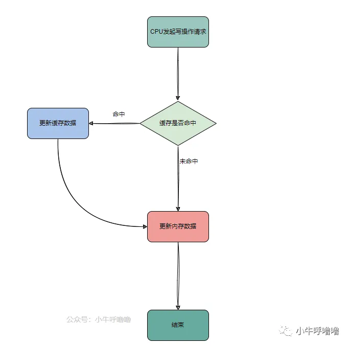
该策略具备逻辑简单、数据可靠性高的优势,但存在性能短板。由于每次写操作均需交互主存,降低了缓存的高速读写性能,仅读操作可发挥缓存加速作用。
1.2 Write Back 写回策略
Write Back 写回策略又称延迟写入策略,相较于写直达策略,可有效减少主存交互次数,是现代 CPU Cache 的主流写入方案。该策略的逻辑为:CPU 向缓存写入数据时,仅更新 Cache 内部数据,同时为对应 Cache Line 标记 dirty 脏位,标识当前缓存数据与主存数据不一致,不实时同步主存数据,将主存写入操作延迟执行。
仅当对应 Cache Line 需替换加载新数据时,系统才会将该脏状态 Cache Line 的数据回写至主存,完成数据同步。
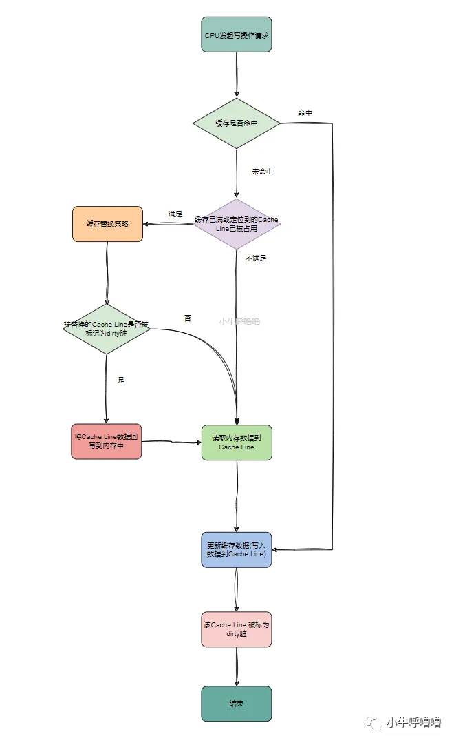
写回策略的优势为降低主存读写频次、提升 CPU 运行效率,缺点是硬件实现逻辑更为复杂。其完整执行流程如下:
- CPU 发起数据写入请求,若缓存命中,直接更新 Cache 数据,并将对应 Cache Line 标记为脏状态;
- 若缓存未命中,系统判定缓存空间已满或目标 Cache Line 已被占用时,触发缓存替换策略;
- 若待替换 Cache Line 为脏状态,优先将其数据回写至主存,再写入新数据并更新脏位标记;
- 若待替换 Cache Line 为干净状态、缓存空间未满或目标位置未被占用,直接写入新数据并标记脏位,等待下一次硬件请求。
二、主流缓存替换策略
缓存空间容量有限,当新数据加载且缓存空间耗尽时,需通过替换策略淘汰旧缓存数据,为新数据提供存储空间。工业界主流替换策略包含 RR、FIFO、LRU 三种。
2.1 RR 随机替换策略
随机替换策略(Random Replacement,RR)通过随机选取缓存块完成数据替换,硬件实现逻辑极简。在大容量缓存场景下,该策略可有效降低替换频次、提升缓存命中率。
其存在一定局限性:未利用计算机数据访问局部性原理,无法针对性优化缓存命中率;小容量缓存场景下易出现频繁替换问题,导致缓存运行效率不稳定。
2.2 FIFO 先进先出策略
先进先出策略(First-In-First-Out,FIFO)依据数据进入缓存的时间顺序执行替换,每次淘汰最早载入缓存的数据,遵循"先入先淘汰"的调度规则。
该算法硬件实现逻辑简单,适配短期临时缓存数据的存储场景,不适用于长期高频数据缓存场景,缓存内的数据易出现过期失效问题。当缓存容量不足时,该算法会产生频繁的数据替换行为,降低缓存整体运行效率。
FIFO 算法存在典型的 Belady 贝莱迪现象:在特定数据访问序列下,缓存容量增大后,缓存命中率出现反向下降的情况。该现象发生概率较低,但会对缓存调度稳定性造成持续性影响。
1969 年,贝莱迪在针对 FIFO 算法的研究中验证了该异常现象:在特定页面请求序列下,配置 4 个页框的缺页次数高于配置 3 个页框的缺页次数。核心成因是,同一时刻 4 页框缓存存储的页面集合,无法完全包含 3 页框缓存的页面集合,两类缓存页面集合不构成严格的超集与子集关系,最终导致大容量缓存的命中率反向降低。
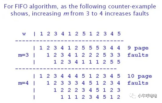
2.3 LRU 最近最少使用策略
最近最少使用策略(Least-Recently-Used,LRU)基于数据访问局部性原理设计,规则为:依据数据访问时间筛选替换对象,以此提升缓存命中率。
该策略适配多数业务场景,硬件兼容性强、性能稳定,且不会产生 Belady 现象,小容量缓存的数据集合始终为大容量缓存数据集合的子集。其局限性为:缓存容量达到阈值后,旧数据清理不当易引发性能波动,无法实现最优缓存调度效果。
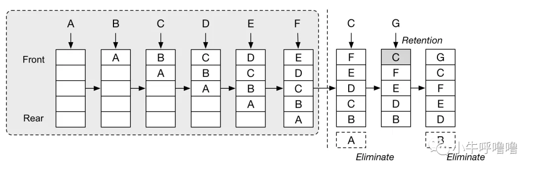
除上述三种主流策略外,业界还存在 LFU、2Q、MQ、ARC 等优化型缓存替换算法,可根据业务场景按需选用。
三、多处理器 CPU 缓存一致性问题与解决方案
现代 CPU 普遍采用多处理器架构,各处理器均配置独立的 L1、L2 缓存,共享 L3 缓存与主存。单核架构的写直达、写回策略仅能解决单缓存与主存的数据同步问题,无法处理多处理器处理器场景下的跨处理器缓存数据不一致问题,需专用一致性机制保障全局数据同步。
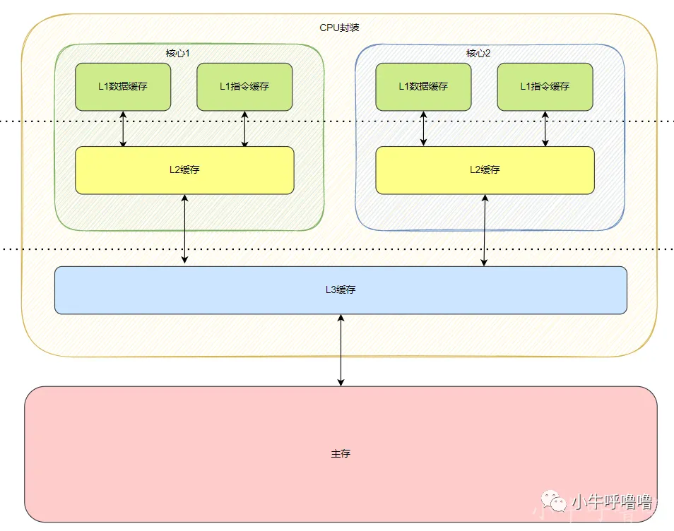
当前多处理器缓存一致性的主流实现方案分为两类:基于总线监听的一致性策略、基于目录的一致性策略。
3.1 基于总线监听的一致性策略
基于总线监听的一致性策略又称总线嗅探(Bus Snooping),依托系统总线实现全处理器缓存数据同步,工作机制如下:
- 任意处理器修改本地缓存数据时,通过系统总线向所有处理器广播数据更新事件;
- 所有处理器持续监听总线广播信号,检测自身缓存是否存在对应数据副本,并执行同步操作,保障全局缓存一致性。
总线监听机制包含两种协议:
- 写更新协议(write-update):单一缓存数据更新后,同步广播更新所有处理器的对应数据副本,一致性效果实时性强,但总线数据传输开销较高;
- 写失效协议(write-invalidate):单一缓存数据更新后,将其他处理器的对应数据副本标记为无效状态,仅保留一份有效可读写数据副本。该协议总线资源开销更小,为工业界通用方案。
3.2 基于目录的一致性策略
基于目录的一致性策略通过维护专用目录数据结构,记录各缓存数据副本的归属处理器与运行状态。相较于总线全局广播模式,该策略无需向所有处理器推送同步信号,仅根据目录记录定向更新对应处理器的缓存状态,可降低总线带宽消耗,具备更强的架构扩展性。
该策略包含 SI、MSI、MESI 等迭代方案,其中 MESI 协议是目前主流的多处理器缓存一致性协议。
四、MESI 缓存一致性协议
MESI 协议是基于失效机制的缓存一致性协议,融合总线嗅探与目录状态管理双重机制,在保障多处理器缓存数据一致性的同时,合理管控总线资源占用。
缓存一致性需满足两项约束条件:
- 写传播(Write Propagation):单一处理器的缓存数据更新,可同步传播至所有处理器的对应缓存副本;
- 事务顺序化(Transaction Serialization):各处理器观测到的全局读写事务执行顺序完全一致,保障并发场景下的数据可见性与有序性。
4.1 MESI 四大状态定义
MESI 协议为每个 Cache Line 定义四种互斥状态,覆盖缓存数据的所有运行场景:
- M(Modified,已修改):当前 Cache Line 数据已被本地处理器修改,未同步至主存,本地缓存数据与主存数据不一致;
- E(Exclusive,独占):当前 Cache Line 仅被本地处理器占用,缓存数据与主存数据完全一致;
- S(Shared,共享):当前 Cache Line 被多个处理器共享占用,所有缓存副本与主存数据完全一致;
- I(Invalidated,已失效):当前 Cache Line 数据无效,无有效可读可写数据。
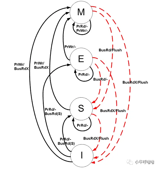
MESI 协议本质为有限状态机,所有状态转换由本地处理器操作、总线全局事件两类场景触发。
4.2 事件分类
MESI 协议的状态转换依赖两类标准化事件:
1. 本地处理器事件
- PrRd:处理器发起缓存块读请求;
- PrWr:处理器发起缓存块写请求。
2. 总线全局监听事件
- BusRd:监听到其他处理器的缓存块读请求;
- BusRdX:监听到其他处理器的非占有缓存块写请求;
- BusUpgr:监听到其他处理器的自有缓存块写请求;
- Flush:触发缓存块数据回写主存操作;
- FlushOpt:触发缓存间数据传输操作,将本地缓存数据推送至总线供其他处理器读取。
4.3 状态兼容约束
在 MESI 协议中,同内存地址的多处理器 Cache Line 存在严格的状态兼容约束,用于保障全局缓存数据一致性。独占类状态 M(Modified)与 E(Exclusive)具备排他属性,不允许与其他处理器的有效缓存状态共存;当任意一个处理器的同地址 Cache Line 处于 S(Shared)共享有效状态时,其余所有处理器对应的同地址 Cache Line,仅可维持 S 共享状态或 I 失效状态,不存在其他合法状态组合。
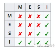
以变量数据缓存场景为例:若 Cache 1 中存储变量 x = 0 x=0 x=0 的 Cache Line 为 S 状态,则 Cache 2、Cache 3 等其余处理器中对应变量 x x x 的 Cache Line,仅能为 S 状态或 I 状态。
4.4 完整状态转换逻辑
结合各类事件与状态定义,可完整梳理 MESI 协议的状态流转规则,覆盖所有读写场景的状态变更与总线操作。
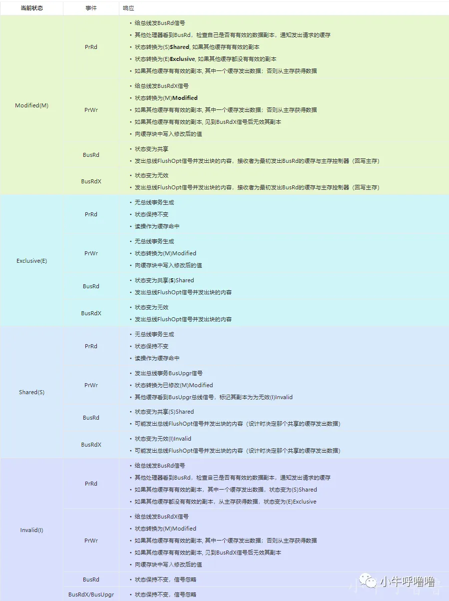
可通过交互式平台 VivioJS 直观观测 MESI 协议运行机制,实时模拟内存、缓存数据与状态的动态变化。
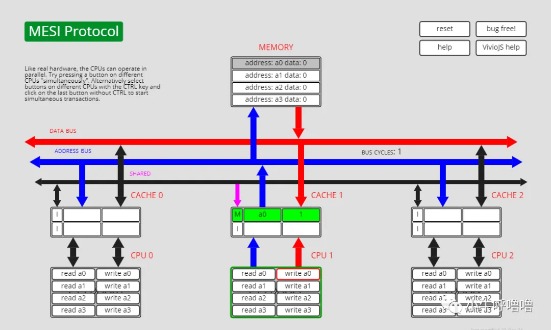
五、MESI 协议性能优化机制
标准 MESI 协议需等待全局总线同步应答后,方可完成缓存读写操作,存在较高的总线延时,会造成 CPU 算力闲置。为优化运行效率,硬件层面引入 Store Buffer 写缓冲区与 Invalidate Queue 失效队列两类优化机制。
5.1 Store Buffer 写缓冲区
当处理器向无效状态缓存写入数据时,无需阻塞等待全局独占权确认应答,可直接将写入指令与数据存入 Store Buffer,即刻执行后续运算任务。总线同步、权限申请、缓存更新等低速操作均由写缓冲区异步完成。
该机制可消除 CPU 等待延时,但会引发数据可见性偏差:本地处理器可提前感知写入操作,其他处理器需等待缓冲区数据同步至缓存后,方可读取最新数据。
5.2 Invalidate Queue 失效队列
处理器接收总线失效请求时,无需暂停当前运算任务处理失效指令,可即刻返回应答信号,同时将失效请求存入 Invalidate Queue,待硬件空闲时批量处理队列中的失效任务。
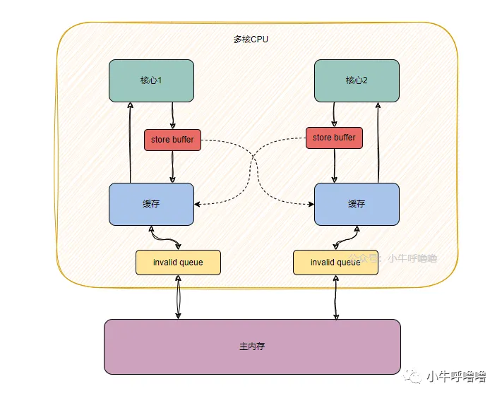
该机制降低了总线交互延时,但会产生状态不一致问题:发起写入的处理器默认其他处理器缓存已失效,但若失效队列未及时处理任务,其他处理器仍可读取旧缓存数据。
六、内存屏障机制
Store Buffer 与 Invalidate Queue 的异步优化机制提升了 CPU 运行效率,但破坏了缓存数据的实时一致性与事务有序性。为修正该问题,硬件引入内存屏障机制,强制同步缓存状态与数据,保障并发场景的数据可靠性。
内存屏障分为两类,适配不同同步场景:
- 写屏障(Store Barrier):强制刷新 Store Buffer 内的缓存数据,将异步写入的数据同步至全局缓存,保障所有处理器可感知最新写入结果;
- 读屏障(Read Barrier):强制清空并处理 Invalidate Queue 内所有失效请求,确保本地处理器读取的数据为全局最新有效数据。
内存屏障是并发编程可见性、有序性的底层硬件支撑,也是 Java volatile 关键字的底层实现原理之一。
参考资料:
徐文浩 《深入浅出计算机组成原理》
Memory management and Virtual memory
https://en.wikipedia.org/wiki/MESI_protocol
https://en.wikipedia.org/wiki/Cache_coherence
https://zhuanlan.zhihu.com/p/591436083
https://lotabout.me/2022/MESI-Protocol-Introduction
reference
-
What is cache memory - Gary explains - 2016
https://www.androidauthority.com/what-is-cache-memory-gary-explains-681747/
-
Use explicit data prefetching to faster process your data structure - 2020
https://johnnysswlab.com/use-explicit-data-prefetching-to-faster-process-your-data-structure/
-
Make your programs run faster by better using the data cache - 2020
https://johnysswlab.com/make-your-programs-run-faster-by-better-using-the-data-cache/
-
CPU Cache 是如何映射与寻址的?
-
突破计算机性能瓶颈的利器 CPU Cache
-
CPU Cache 是如何保证缓存一致性?