注:本文为 "计算机内存系统" 相关合辑。
英文引文,机翻未校。
中文引文,略作重排。
图片清晰度受引文原图所限。
如有内容异常,请看原文。
What Your Computer Does While You Wait
等待期间,你的计算机在做什么
Dec 1st, 2008
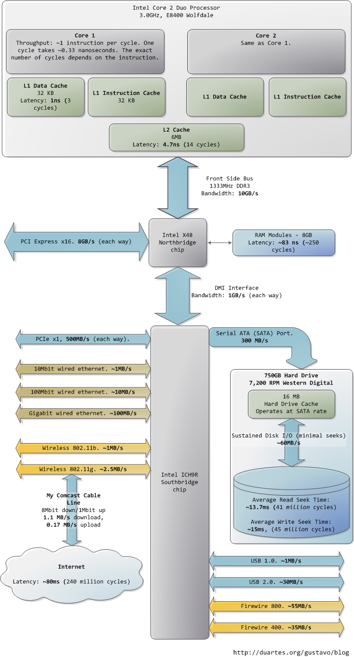
This post takes a look at the speed --- latency and throughput --- of various subsystems in a modern commodity PC, an Intel Core 2 Duo at 3.0 GHz. I hope to give a feel for the relative speed of each component and a cheatsheet for back-of-the-envelope performance calculations. I've tried to show real-world throughputs (the sources are posted as a comment) rather than theoretical maximums. Time units are nanoseconds (ns, 10 − 9 10^{-9} 10−9 seconds), milliseconds (ms, 10 − 3 10^{-3} 10−3 seconds), and seconds (s). Throughput units are in megabytes and gigabytes per second. Let's start with CPU and memory, the north of the northbridge:
本文考察一台现代商用 PC(Intel Core 2 Duo @ 3.0 GHz)中各子系统的速度------延迟与吞吐量。我希望让读者对各组件的相对速度有一个直观感受,并提供一份用于粗略性能估算的速查表。我尽量给出实际吞吐量,而非理论最大值。时间单位为纳秒(ns, 10 − 9 10^{-9} 10−9 s)、毫秒(ms, 10 − 3 10^{-3} 10−3 s)和秒(s)。吞吐量单位为 MB/s 与 GB/s。让我们从 CPU 与内存开始,即北桥以北:
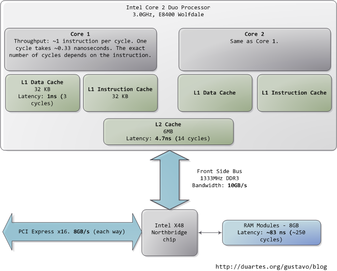
The first thing that jumps out is how absurdly fast our processors are. Most simple instructions on the Core 2 take one clock cycle to execute, hence a third of a nanosecond at 3.0 GHz. For reference, light only travels ~4 inches (10 cm) in the time taken by a clock cycle. It's worth keeping this in mind when you're thinking of optimization --- instructions are comically cheap to execute nowadays.
首先映入眼帘的是我们的处理器速度快得惊人。Core 2 上大多数简单指令仅需 一个时钟周期 即可执行,因此在 3.0 GHz 下仅需 三分之一纳秒。作为参照,光在一个时钟周期内只前进约 4 英寸(10 cm)。在考虑优化时请记住这一点------如今执行指令的代价低得可笑。
As the CPU works away, it must read from and write to system memory, which it accesses via the L1 and L2 caches. The caches use static RAM, a much faster (and expensive) type of memory than the DRAM memory used as the main system memory. The caches are part of the processor itself and for the pricier memory we get very low latency. One way in which instruction-level optimization is still very relevant is code size. Due to caching, there can be massive performance differences between code that fits wholly into the L1/L2 caches and code that needs to be marshalled into and out of the caches as it executes.
CPU 在工作的过程中,必须读写系统内存,而这要通过 L1 和 L2 缓存完成。缓存使用静态 RAM(SRAM),它比用作主存的 DRAM 更快(也更昂贵)。缓存是处理器本身的一部分,我们付出了更高的存储代价,换来了极低的延迟。指令级优化仍然非常相关的一个方面是代码体积。由于缓存的存在,完全容纳在 L1/L2 缓存中的代码与执行过程中需要不断调入调出缓存的代码之间,可能存在巨大的性能差异。
Normally when the CPU needs to touch the contents of a memory region they must either be in the L1/L2 caches already or be brought in from the main system memory. Here we see our first major hit, a massive ~250 cycles of latency that often leads to a stall , when the CPU has no work to do while it waits. To put this into perspective, reading from L1 cache is like grabbing a piece of paper from your desk (3 seconds), L2 cache is picking up a book from a nearby shelf (14 seconds), and main system memory is taking a 4-minute walk down the hall to buy a Twix bar.
通常,当 CPU 需要访问某内存区域的内容时,这些内容要么已经在 L1/L2 缓存中,要么必须从主存调入。在这里我们遭遇了第一个重大打击:巨大的约 250 个时钟周期的延迟,这往往导致 停顿(stall),即 CPU 在等待期间无事可做。打个比方:从 L1 缓存读取就像从桌面上拿起一张纸(3 秒),从 L2 缓存读取就像从附近书架上取一本书(14 秒),而从主存读取则像下楼走 4 分钟去大厅买一根 Twix 巧克力棒。
The exact latency of main memory is variable and depends on the application and many other factors. For example, it depends on the CAS latency and specifications of the actual RAM stick that is in the computer. It also depends on how successful the processor is at prefetching --- guessing which parts of memory will be needed based on the code that is executing and having them brought into the caches ahead of time.
主存的精确延迟是可变的,取决于应用程序及诸多其他因素。例如,它取决于实际安装在计算机中的内存条的 CAS 延迟及规格。它还取决于处理器的预取(prefetching)效果------即根据正在执行的代码预测接下来需要哪些内存区域,并提前将其载入缓存。
Looking at L1/L2 cache performance versus main memory performance, it is clear how much there is to gain from larger L2 caches and from applications designed to use it well. For a discussion of all things memory, see Ulrich Drepper's What Every Programmer Should Know About Memory (pdf), a fine paper on the subject.
对比 L1/L2 缓存与主存的性能,不难看出更大的 L2 缓存以及善于利用缓存的应用程序能带来多大的收益。关于内存的一切讨论,请参阅 Ulrich Drepper 的论文 What Every Programmer Should Know About Memory(PDF),这是一篇关于该主题的佳作。
People refer to the bottleneck between CPU and memory as the [von Neumann bottleneck. Now, the front side bus bandwidth, ~10 GB/s, actually looks decent. At that rate, you could read all of 8 GB of system memory in less than one second or read 100 bytes in 10 ns. Sadly this throughput is a theoretical maximum (unlike most others in the diagram) and cannot be achieved due to delays in the main RAM circuitry. Many discrete wait periods are required when accessing memory. The electrical protocol for access calls for delays after a memory row is selected, after a column is selected, before data can be read reliably, and so on. The use of capacitors calls for periodic refreshes of the data stored in memory lest some bits get corrupted, which adds further overhead. Certain consecutive memory accesses may happen more quickly but there are still delays, and more so for random access. Latency is always present.
人们将 CPU 与内存之间的瓶颈称为冯 · 诺依曼瓶颈(von Neumann bottleneck)。前端总线带宽约为 10 GB/s,看起来还不错。按照这个速率,你可以在不到 1 秒内读完 8 GB 的系统内存,或者在 10 ns 内读取 100 字节。遗憾的是,这一吞吐量是理论最大值(与图中大多数其他值不同),由于主存电路中的延迟,它实际上无法达到。访问内存时需要许多离散的等待周期。访问的电气协议要求在行选通后、列选通后、数据可靠读取前等时刻插入延迟。电容的使用要求定期刷新内存中存储的数据,以免某些位发生损坏,这进一步增加了开销。某些连续的内存访问可能更快,但延迟依然存在,随机访问时尤其如此。延迟无处不在。
Down in the southbridge we have a number of other buses (e.g. , PCIe, USB) and peripherals connected:
在南桥中,我们连接了若干其他总线(例如 PCIe、USB)及外设:
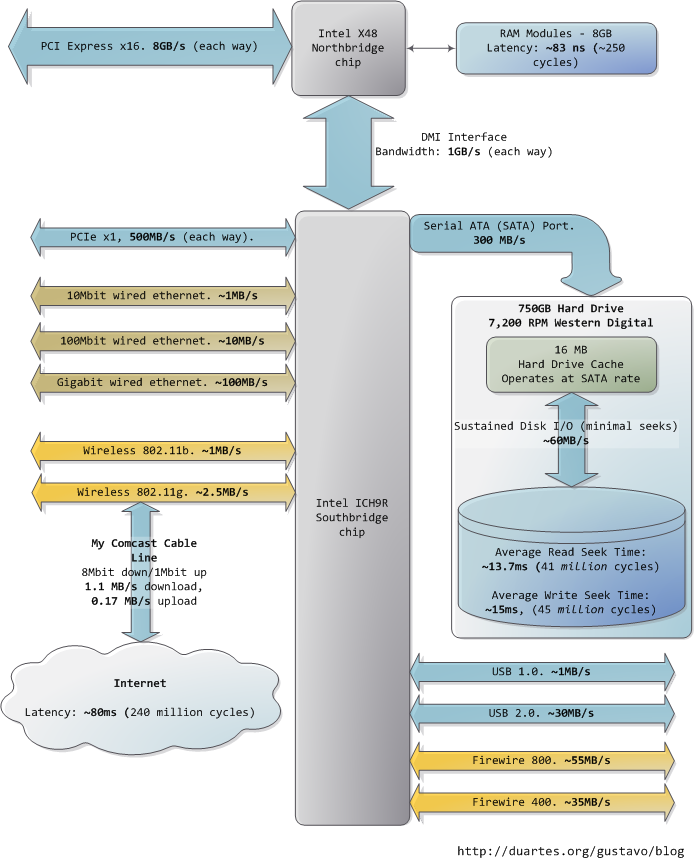
Sadly the southbridge hosts some truly sluggish performers, for even main memory is blazing fast compared to hard drives. Keeping with the office analogy, waiting for a hard drive seek is like leaving the building to roam the earth for one year and three months . This is why so many workloads are dominated by disk I/O and why database performance can drive off a cliff once the in-memory buffers are exhausted. It is also why plentiful RAM (for buffering) and fast hard drives are so important for overall system performance.
遗憾的是,南桥中驻留着一些真正慢吞吞的设备,因为与硬盘相比,连主存都快得惊人。沿用办公室比喻,等待一次硬盘寻道就像离开大楼去地球上漫游 一年零三个月。这就是为什么如此多的工作负载被磁盘 I/O 主导,以及为什么数据库性能会在内存缓冲区耗尽后断崖式下跌。这也是为什么充足的 RAM(用于缓冲)和高速硬盘对整体系统性能至关重要。
While the "sustained" disk throughput is real in the sense that it is actually achieved by the disk in real-world situations, it does not tell the whole story. The bane of disk performance are seeks, which involve moving the read/write heads across the platter to the right track and then waiting for the platter to spin around to the right position so that the desired sector can be read. Disk RPMs refer to the speed of rotation of the platters: the faster the RPMs, the less time you wait on average for the rotation to give you the desired sector, hence higher RPMs mean faster disks. A cool place to read about the impact of seeks is the paper where a couple of Stanford grad students describe the [Anatomy of a Large-Scale Hypertextual Web Search Engine (pdf).
虽然"持续"磁盘吞吐量在真实世界场景中确实由磁盘实际达到,但它并未讲述全部故事。磁盘性能的祸根是寻道(seek),它涉及将读写头移动到盘片上的正确磁道,然后等待盘片旋转到正确位置以便读取目标扇区。磁盘 RPM 指盘片的旋转速度:RPM 越高,平均等待旋转到目标扇区的时间越短,因此更高的 RPM 意味着更快的磁盘。想了解寻道影响的精彩读物,请参阅两位斯坦福研究生描述大型超文本网络搜索引擎的剖析的论文。
When the disk is reading one large continuous file it achieves greater sustained read speeds due to the lack of seeks. Filesystem defragmentation aims to keep files in continuous chunks on the disk to minimize seeks and boost throughput. When it comes to how fast a computer feels, sustained throughput is less important than seek times and the number of random I/O operations (reads/writes) that a disk can do per time unit. Solid state disks can make for a [great option here.
当磁盘读取一个大型连续文件时,由于缺乏寻道,它能获得更高的持续读取速度。文件系统碎片整理的目的是将文件保持在磁盘上的连续块中,以最小化寻道并提升吞吐量。就计算机的"感觉速度"而言,持续吞吐量不如寻道时间和磁盘每时间单位可执行的随机 I/O 操作数(读/写)重要。固态硬盘(SSD)在此可以成为一个绝佳选择。
Hard drive caches also help performance. Their tiny size --- a 16 MB cache in a 750 GB drive covers only 0.002% of the disk --- suggest they're useless, but in reality their contribution is allowing a disk to [queue up writes and then perform them in one bunch, thereby allowing the disk to plan the order of the writes in a way that --- surprise --- minimizes seeks. Reads can also be grouped in this way for performance, and both the OS and the drive firmware engage in these optimizations.
硬盘缓存也有助于提升性能。它们的体积很小------750 GB 硬盘中的 16 MB 缓存仅占磁盘容量的 0.002%------看似毫无用处,但实际上它们的贡献在于允许磁盘将写入操作排队,然后一次性执行,从而让磁盘能够以------惊喜------最小化寻道的方式规划写入顺序。读取也可以按这种方式分组以提升性能,操作系统和硬盘固件都会执行这类优化。
Finally, the diagram has various real-world throughputs for networking and other buses. Firewire is shown for reference but is not available natively in the Intel X48 chipset. It's fun to think of the Internet as a computer bus. The latency to a fast website (say, google.com) is about 45 ms, comparable to hard drive seek latency. In fact, while hard drives are 5 orders of magnitude removed from main memory, they're in the same magnitude as the Internet. Residential bandwidth still lags behind that of sustained hard drive reads, but the 'network is the computer' in a pretty literal sense now. What happens when the Internet is faster than a hard drive?
最后,图中还展示了网络及其他总线的各种实际吞吐量。Firewire 仅作参考,Intel X48 芯片组并不原生支持。把互联网想象成计算机总线是一件有趣的事。访问一个快速网站(例如 google.com)的延迟约为 45 ms,与硬盘寻道延迟相当。事实上,虽然硬盘与主存之间相差 5 个数量级,但它们与互联网处于同一数量级。家庭带宽仍落后于硬盘的持续读取速度,但"网络即计算机"如今已是相当字面上的含义。当互联网比硬盘更快时会发生什么?
I hope this diagram is useful. It's fascinating for me to look at all these numbers together and see how far we've come. Sources are posted as a comment. I posted a full diagram showing both north and south bridges [here if you're interested.
希望这张图对你有用。对我来说,将这些数字放在一起看,并审视我们已取得的进步,是令人着迷的。来源已在评论中贴出。如果你感兴趣,我在此处发布了一张展示南北桥的完整图表。
Cache: a place for concealment and safekeeping
缓存:隐匿与暂存之地
Jan 12th, 2009
This post shows briefly how CPU caches are organized in modern Intel processors. Cache discussions often lack concrete examples, obfuscating the simple concepts involved. Or maybe my pretty little head is slow. At any rate, here's half the story on how a Core 2 L1 cache is accessed:
本文简要展示了现代 Intel 处理器中 CPU 缓存的组织方式。关于缓存的讨论往往缺乏具体实例,使得涉及的一些简单概念变得扑朔迷离。也许是我可爱的小脑瓜反应慢。无论如何,下面是 Core 2 L1 缓存访问方式的前半部分故事:
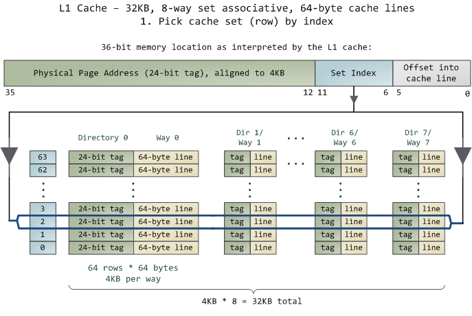
The unit of data in the cache is the line , which is just a contiguous chunk of bytes in memory. This cache uses 64-byte lines. The lines are stored in cache banks or ways , and each way has a dedicated directory to store its housekeeping information. You can imagine each way and its directory as columns in a spreadsheet, in which case the rows are the sets . Then each cell in the way column contains a cache line, tracked by the corresponding cell in the directory. This particular cache has 64 sets and 8 ways, hence 512 cells to store cache lines, which adds up to 32 KB of space.
缓存中的数据单位是 缓存行(line) ,即内存中一段连续的字节块。该缓存使用 64 字节的行。这些行存储在缓存体或 路(way) 中,每一路都有一个专用的 目录(directory) 来存储其管理信息。你可以把每一路及其目录想象成电子表格中的列,那么行就是 组(set)。然后,way 列中的每个单元格包含一条缓存行,由目录中对应的单元格跟踪。这个特定缓存有 64 个组、8 路,因此有 512 个用于存储缓存行的单元格,总计 32 KB 空间。
In this cache's view of the world, physical memory is divided into 4 KB physical pages. Each page has 4 KB / 64 bytes == 64 cache lines in it. When you look at a 4 KB page, bytes 0 through 63 within that page are in the first cache line, bytes 64--127 in the second cache line, and so on. The pattern repeats for each page, so the 3rd line in page 0 is different than the 3rd line in page 1.
在该缓存的视角中,物理内存被划分为 4 KB 的物理页。每页包含 64 条缓存行。观察一个 4 KB 页,页内字节 0 到 63 位于第一条缓存行,字节 64 到 127 位于第二条缓存行,以此类推。该模式在每页中重复,因此第 0 页的第 3 条缓存行与第 1 页的第 3 条缓存行是不同的。
In a fully associative cache any line in memory can be stored in any of the cache cells. This makes storage flexible, but it becomes expensive to search for cells when accessing them. Since the L1 and L2 caches operate under tight constraints of power consumption, physical space, and speed, a fully associative cache is not a good trade off in most scenarios.
在 全相联缓存(fully associative cache) 中,内存中的任意一行都可以存储在任意缓存单元中。这使得存储非常灵活,但访问时搜索单元会变得昂贵。由于 L1 和 L2 缓存受到功耗、物理空间和速度等严格限制,全相联缓存在大多数场景下并非良好的折中方案。
Instead, this cache is set associative , which means that a given line in memory can only be stored in one specific set (or row) shown above. So the first line of any physical page (bytes 0--63 within a page) must be stored in row 0, the second line in row 1, etc. Each row has 8 cells available to store the cache lines it is associated with, making this an 8-way associative set. When looking at a memory address, bits 11--6 determine the line number within the 4 KB page and therefore the set to be used. For example, physical address 0x800010a0 has 000010 in those bits so it must be stored in set 2.
相反,该缓存是 组相联(set associative) 的,这意味着内存中给定的一行只能存储在上面所示的一个特定组(或行)中。因此,任意物理页 的第一行(页内字节 0--63)必须 存储在第 0 行,第二行存储在第 1 行,以此类推。每行有 8 个单元格可用于存储与其关联的缓存行,从而形成一个 8 路组相联集。查看内存地址时,第 11--6 位决定了 4 KB 页内的行号,从而确定了要使用的组。例如,物理地址 0x800010a0 在这些位上的值为 000010,因此它必须存储在第 2 组。
But we still have the problem of finding which cell in the row holds the data, if any. That's where the directory comes in. Each cached line is tagged by its corresponding directory cell; the tag is simply the number for the page where the line came from. The processor can address 64 GB of physical RAM, so there are 64 GB / 4 KB == 2 24 2^{24} 224 of these pages and thus we need 24 bits for our tag. Our example physical address 0x800010a0 corresponds to page number 524,289. Here's the second half of the story:
但我们仍然面临一个问题:如果数据存在,要找出该行中 哪个 单元格保存了数据。这就是目录发挥作用的地方。每条缓存行都被其对应的目录单元格 标记(tag) ;标记就是该行来源页的页号。处理器可寻址 64 GB 物理 RAM,因此共有 2 24 2^{24} 224 个页,我们需要 24 位作为标记。示例物理地址 0x800010a0 对应的页号为 524,289。下面是故事的后半部分:
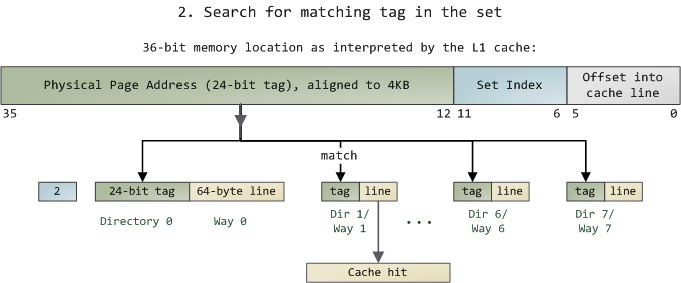
Since we only need to look in one set of 8 ways, the tag matching is very fast; in fact, electrically all tags are compared simultaneously, which I tried to show with the arrows. If there's a valid cache line with a matching tag, we have a cache hit. Otherwise, the request is forwarded to the L2 cache, and failing that to main system memory. Intel builds large L2 caches by playing with the size and quantity of the ways, but the design is the same. For example, you could turn this into a 64 KB cache by adding 8 more ways. Then increase the number of sets to 4096 and each way can store 256 KB. These two modifications would deliver a 4 MB L2 cache. In this scenario, you'd need 18 bits for the tags and 12 for the set index; the physical page size used by the cache is equal to its way size.
由于我们只需查看一个组中的 8 路,标记匹配非常快;事实上,从电气角度所有标记是同时比较的,我试图用箭头表示这一点。如果存在一条有效缓存行且标记匹配,则发生缓存命中(cache hit)。否则,请求被转发到 L2 缓存,若仍未命中则转至主存。Intel 通过调整路的大小和数量来构建大型 L2 缓存,但设计原理相同。例如,你可以通过增加 8 路将其变为 64 KB 缓存。然后将组数增加到 4096,每路可存储 256 KB。这两项修改将得到一个 4 MB 的 L2 缓存。在此场景中,标记需要 18 位,组索引需要 12 位;缓存使用的物理页大小等于其路大小。
If a set fills up, then a cache line must be evicted before another one can be stored. To avoid this, performance-sensitive programs try to organize their data so that memory accesses are evenly spread among cache lines. For example, suppose a program has an array of 512-byte objects such that some objects are 4 KB apart in memory. Fields in these objects fall into the same lines and compete for the same cache set. If the program frequently accesses a given field (e.g. , the vtable by calling a virtual method), the set will likely fill up and the cache will start trashing as lines are repeatedly evicted and later reloaded. Our example L1 cache can only hold the vtables for 8 of these objects due to set size. This is the cost of the set associativity trade-off: we can get cache misses due to set conflicts even when overall cache usage is not heavy. However, due to the relative speeds in a computer, most apps don't need to worry about this anyway.
如果一个组满了,则必须先驱逐一条缓存行才能存储新的。为避免这种情况,对性能敏感的程序会尝试组织数据,使内存访问均匀分布在各缓存行中。例如,假设一个程序有一个 512 字节对象的数组,其中某些对象在内存中相距 4 KB。这些对象中的字段会落入同一行并竞争同一缓存组。如果程序频繁访问某个字段(例如,通过调用虚函数的 vtable),该组很可能填满,缓存将开始抖动(trashing),因为行被反复驱逐后又重新加载。示例中的 L1 缓存由于组大小限制,只能容纳 8 个此类对象的 vtable。这就是组相联折中的代价:即使整体缓存使用率不高,我们也可能因组冲突而遭遇缓存未命中。然而,鉴于计算机中各存储层次的相对速度,大多数应用程序无论如何都无需担心这一点。
A memory access usually starts with a linear (virtual) address, so the L1 cache relies on the paging unit to obtain the physical page address used for the cache tags. By contrast, the set index comes from the least significant bits of the linear address and is used without translation (bits 11--6 in our example). Hence the L1 cache is physically tagged but virtually indexed , helping the CPU to parallelize lookup operations. Because the L1 way is never bigger than an MMU page, a given physical memory location is guaranteed to be associated with the same set even with virtual indexing. L2 caches, on the other hand, must be physically tagged and physically indexed because their way size can be bigger than MMU pages. But then again, by the time a request gets to the L2 cache the physical address was already resolved by the L1 cache, so it works out nicely.
内存访问通常始于线性(虚拟)地址,因此 L1 缓存依赖分页单元获取用于缓存标记的物理页地址。相比之下,组索引来自线性地址的最低有效位,无需转换即可使用(示例中的第 11--6 位)。因此 L1 缓存是 物理标记(physically tagged) 但 虚拟索引(virtually indexed) 的,这有助于 CPU 并行化查找操作。由于 L1 路大小从不超过 MMU 页大小,即使使用虚拟索引,给定物理内存位置也保证关联到同一组。另一方面,L2 缓存必须是物理标记且物理索引的,因为其路大小可能超过 MMU 页大小。但话说回来,当请求到达 L2 缓存时,物理地址已由 L1 缓存解析完毕,因此一切顺理成章。
Finally, a directory cell also stores the state of its corresponding cached line. A line in the L1 code cache is either Invalid or Shared (which means valid, really). In the L1 data cache and the L2 cache, a line can be in any of the 4 MESI states: Modified, Exclusive, Shared, or Invalid. Intel caches are inclusive : the contents of the L1 cache are duplicated in the L2 cache. These states will play a part in later posts about threading, locking, and that kind of stuff. Next time we'll look at the front side bus and how memory access really works. This is going to be memory week.
最后,目录单元格还存储其对应缓存行的 状态(state) 。L1 指令缓存中的一行要么为 Invalid,要么为 Shared(实际意味着有效)。在 L1 数据缓存和 L2 缓存中,一行可以处于 4 种 MESI 状态之一:Modified、Exclusive、Shared 或 Invalid。Intel 缓存是 包容式(inclusive) 的:L1 缓存的内容在 L2 缓存中有副本。这些状态将在后续关于线程、锁等主题的文章中发挥作用。下次我们将考察前端总线以及内存访问 真正 的工作原理。这将是一个内存专题周。
Update : Dave brought up direct-mapped caches in a comment below. They're basically a special case of set-associative caches that have only one way. In the trade-off spectrum, they're the opposite of fully associative caches: blazing fast access, lots of conflict misses.
更新:Dave 在下方评论中提到了直接映射缓存(direct-mapped cache)。它们本质上是只有一路的组相联缓存的特例。在折中谱系中,它们与全相联缓存正好相反:访问极快,但冲突未命中很多。
Anatomy of a Program in Memory
程序内存剖析
Jan 27th, 2009
Memory management is the heart of operating systems; it is crucial for both programming and system administration. In the next few posts I'll cover memory with an eye towards practical aspects, but without shying away from internals. While the concepts are generic, examples are mostly from Linux and Windows on 32-bit x86. This first post describes how programs are laid out in memory.
内存管理是操作系统的核心;它对编程和系统管理都至关重要。在接下来的几篇文章中,我将从实用角度出发探讨内存,同时也不会回避底层实现。虽然这些概念具有通用性,但示例主要来自 Linux 和 Windows 上的 32 位 x86 架构。本文首先描述程序在内存中的布局方式。
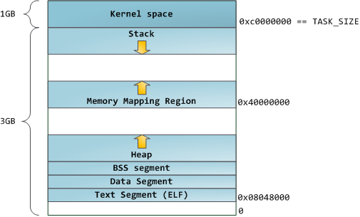
Each process in a multi-tasking OS runs in its own memory sandbox. This sandbox is the virtual address space , which in 32-bit mode is always a 4GB block of memory addresses . These virtual addresses are mapped to physical memory by page tables , which are maintained by the operating system kernel and consulted by the processor. Each process has its own set of page tables, but there is a catch. Once virtual addresses are enabled, they apply to all software running in the machine, including the kernel itself . Thus a portion of the virtual address space must be reserved to the kernel:
多任务操作系统中的每个进程都在自己的内存沙箱中运行。这个沙箱就是虚拟地址空间 ,在 32 位模式下,它始终是一个 4 GB 的内存地址块 。这些虚拟地址通过页表 映射到物理内存,页表由操作系统内核维护,并由处理器查询。每个进程都有自己的页表,但这里有一个问题:一旦启用虚拟地址,它们就适用于机器上运行的所有软件 ,包括内核本身。因此,虚拟地址空间的一部分必须保留给内核:
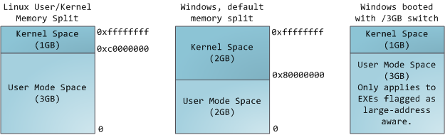
This does not mean the kernel uses that much physical memory, only that it has that portion of address space available to map whatever physical memory it wishes. Kernel space is flagged in the page tables as exclusive to [privileged code (ring 2 or lower), hence a page fault is triggered if user-mode programs try to touch it. In Linux, kernel space is constantly present and maps the same physical memory in all processes. Kernel code and data are always addressable, ready to handle interrupts or system calls at any time. By contrast, the mapping for the user-mode portion of the address space changes whenever a process switch happens:
这并不意味着内核使用了那么多物理内存,而只是意味着它拥有这部分地址空间,可以用来映射它想要的任何物理内存。内核空间在页表中被标记为仅供特权代码(ring 2 或更低)访问,因此如果用户态程序试图触碰它,就会触发页错误。在 Linux 中,内核空间始终存在,并且在所有进程中映射相同的物理内存。内核代码和数据始终可寻址,随时准备处理中断或系统调用。相比之下,用户态地址空间部分的映射在每次进程切换时都会发生变化:
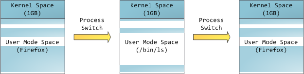
Blue regions represent virtual addresses that are mapped to physical memory, whereas white regions are unmapped. In the example above, Firefox has used far more of its virtual address space due to its legendary memory hunger. The distinct bands in the address space correspond to memory segments like the heap, stack, and so on. Keep in mind these segments are simply a range of memory addresses and have nothing to do with [Intel-style segments. Anyway, here is the standard segment layout in a Linux process:
蓝色区域代表已映射到物理内存的虚拟地址,而白色区域是未映射的。在上面的例子中,Firefox 由于其传奇般的内存消耗,使用了远超其虚拟地址空间的范围。地址空间中不同的带状区域对应于内存段 ,如堆、栈等。请记住,这些段只是内存地址的一个范围,与 Intel 风格的段毫无关系。总之,以下是 Linux 进程中的标准段布局:
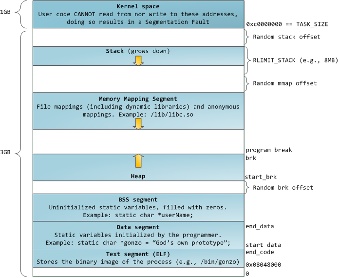
When computing was happy and safe and cuddly, the starting virtual addresses for the segments shown above were exactly the same for nearly every process in a machine. This made it easy to exploit security vulnerabilities remotely. An exploit often needs to reference absolute memory locations: an address on the stack, the address for a library function, etc. Remote attackers must choose this location blindly, counting on the fact that address spaces are all the same. When they are, people get pwned. Thus address space randomization has become popular. Linux randomizes the [stack, [memory mapping segment, and [heap by adding offsets to their starting addresses. Unfortunately the 32-bit address space is pretty tight, leaving little room for randomization and [hampering its effectiveness.
在计算世界还无忧无虑、安全舒适的时候,上图所示各段的起始虚拟地址在机器上几乎每个进程中都完全相同。这使得远程利用安全漏洞变得轻而易举。漏洞利用通常需要引用绝对内存位置:栈上的地址、库函数的地址等。远程攻击者必须盲目地选择这个位置,依赖于所有地址空间都相同这一事实。当它们确实相同时,人们就被攻陷了。因此,地址空间随机化变得流行起来。Linux 通过在起始地址上添加偏移量来随机化栈、内存映射段和堆。不幸的是,32 位地址空间相当紧张,留给随机化的空间很小,从而限制了其有效性。
The topmost segment in the process address space is the stack, which stores local variables and function parameters in most programming languages. Calling a method or function pushes a new stack frame onto the stack. The stack frame is destroyed when the function returns. This simple design, possible because the data obeys strict LIFO order, means that no complex data structure is needed to track stack contents - a simple pointer to the top of the stack will do. Pushing and popping are thus very fast and deterministic. Also, the constant reuse of stack regions tends to keep active stack memory in the cpu caches, speeding up access. Each thread in a process gets its own stack.
进程地址空间中最顶部的段是栈,在大多数编程语言中,它存储局部变量和函数参数。调用方法或函数时,会将一个新的栈帧压入栈。当函数返回时,栈帧被销毁。这种简单的设计之所以可行,是因为数据遵循严格的 LIFO(后进先出)顺序,这意味着不需要复杂的数据结构来跟踪栈内容------一个简单的指向栈顶的指针就足够了。因此,压栈和弹栈非常快速且确定。此外,栈区域的持续复用有助于将活跃的栈内存保留在 CPU 缓存中,从而加快访问速度。进程中的每个线程都有自己的栈。
It is possible to exhaust the area mapping the stack by pushing more data than it can fit. This triggers a page fault that is handled in Linux by expand_stack(), which in turn calls acct_stack_growth() to check whether it's appropriate to grow the stack. If the stack size is below RLIMIT_STACK (usually 8MB), then normally the stack grows and the program continues merrily, unaware of what just happened. This is the normal mechanism whereby stack size adjusts to demand. However, if the maximum stack size has been reached, we have a stack overflow and the program receives a Segmentation Fault. While the mapped stack area expands to meet demand, it does not shrink back when the stack gets smaller. Like the federal budget, it only expands.
有可能通过压入超过栈可容纳的数据量来耗尽栈的映射区域。这会触发一个页错误,在 Linux 中由 expand_stack() 处理,后者又调用 acct_stack_growth() 来检查是否可以增长栈。如果栈大小低于 RLIMIT_STACK(通常为 8 MB),那么栈通常会增长,程序继续愉快地运行,完全不知道刚刚发生了什么。这是栈大小根据需求调整的正常机制。然而,如果已达到最大栈大小,就会发生栈溢出,程序收到段错误。虽然映射的栈区域会扩展以满足需求,但当栈变小时,它不会收缩。就像联邦预算一样,它只增不减。
Dynamic stack growth is the only situation in which access to an unmapped memory region, shown in white above, might be valid. Any other access to unmapped memory triggers a page fault that results in a Segmentation Fault. Some mapped areas are read-only, hence write attempts to these areas also lead to segfaults.
动态栈增长是访问未映射内存区域(上图中的白色区域)可能有效的唯一情况。任何其他对未映射内存的访问都会触发页错误,导致段错误。某些映射区域是只读的,因此对这些区域的写入尝试也会导致段错误。
Below the stack, we have the memory mapping segment. Here the kernel maps contents of files directly to memory. Any application can ask for such a mapping via the Linux mmap() system call (implementation) or CreateFileMapping() / MapViewOfFile() in Windows. Memory mapping is a convenient and high-performance way to do file I/O, so it is used for loading dynamic libraries. It is also possible to create an anonymous memory mapping that does not correspond to any files, being used instead for program data. In Linux, if you request a large block of memory via malloc(), the C library will create such an anonymous mapping instead of using heap memory. 'Large' means larger than MMAP_THRESHOLD bytes, 128 kB by default and adjustable via mallopt().
在栈的下方,是内存映射段。在这里,内核将文件内容直接映射到内存。任何应用程序都可以通过 Linux 的 mmap() 系统调用(实现)或 Windows 的 CreateFileMapping() / MapViewOfFile() 来请求这种映射。内存映射是一种方便且高性能的文件 I/O 方式,因此它被用于加载动态库。也可以创建一种匿名内存映射 ,它不对应任何文件,而是用于程序数据。在 Linux 中,如果你通过 malloc() 请求一大块内存,C 库会创建这样的匿名映射,而不是使用堆内存。"大"指的是超过 MMAP_THRESHOLD 字节,默认值为 128 kB,可通过 mallopt() 调整。
Speaking of the heap, it comes next in our plunge into address space. The heap provides runtime memory allocation, like the stack, meant for data that must outlive the function doing the allocation, unlike the stack. Most languages provide heap management to programs. Satisfying memory requests is thus a joint affair between the language runtime and the kernel. In C, the interface to heap allocation is malloc() and friends, whereas in a garbage-collected language like C# the interface is the new keyword.
说到堆,它是我们深入地址空间的下一个目标。与栈一样,堆提供运行时内存分配,但用于那些必须比执行分配操作的函数存活更久的数据。大多数语言为程序提供堆管理。因此,满足内存请求是语言运行时和内核之间的共同事务。在 C 中,堆分配的接口是 malloc() 及其相关函数,而在像 C# 这样的垃圾回收语言中,接口是 new 关键字。
If there is enough space in the heap to satisfy a memory request, it can be handled by the language runtime without kernel involvement. Otherwise the heap is enlarged via the brk() system call (implementation) to make room for the requested block. Heap management is complex, requiring sophisticated algorithms that strive for speed and efficient memory usage in the face of our programs' chaotic allocation patterns. The time needed to service a heap request can vary substantially. Real-time systems have special-purpose allocators to deal with this problem. Heaps also become fragmented , shown below:
如果堆中有足够的空间来满足内存请求,语言运行时可以在不涉及内核的情况下处理它。否则,堆通过 brk() 系统调用(实现)来扩大,为请求的块腾出空间。堆管理是复杂的,需要精妙的算法,以在程序混乱的分配模式下追求速度和高效的内存使用。满足堆请求所需的时间可能差异很大。实时系统有专门的分配器来处理这个问题。堆也会变得碎片化,如下图所示:
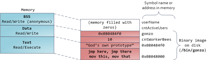
Finally, we get to the lowest segments of memory: BSS, data, and program text. Both BSS and data store contents for static (global) variables in C. The difference is that BSS stores the contents of uninitialized static variables, whose values are not set by the programmer in source code. The BSS memory area is anonymous: it does not map any file. If you say static int cntActiveUsers, the contents of cntActiveUsers live in the BSS.
最后,我们来到内存的最低段:BSS、数据和程序文本。BSS 和数据都存储 C 中静态(全局)变量的内容。区别在于,BSS 存储的是未初始化 的静态变量的内容,其值在源代码中未被程序员设置。BSS 内存区域是匿名的:它不映射任何文件。如果你写 static int cntActiveUsers,cntActiveUsers 的内容就存在于 BSS 中。
The data segment, on the other hand, holds the contents for static variables initialized in source code. This memory area is not anonymous . It maps the part of the program's binary image that contains the initial static values given in source code. So if you say static int cntWorkerBees = 10, the contents of cntWorkerBees live in the data segment and start out as 10. Even though the data segment maps a file, it is a private memory mapping , which means that updates to memory are not reflected in the underlying file. This must be the case, otherwise assignments to global variables would change your on-disk binary image. Inconceivable!
另一方面,数据段保存源代码中已初始化的静态变量的内容。这个内存区域不是匿名的 。它映射程序二进制镜像中包含源代码中给出的初始静态值的部分。所以如果你写 static int cntWorkerBees = 10,cntWorkerBees 的内容就存在于数据段中,初始值为 10。尽管数据段映射了一个文件,但它是私有内存映射,这意味着对内存的更新不会反映到底层文件中。必须如此,否则对全局变量的赋值会改变你的磁盘二进制镜像。不可想象!
The data example in the diagram is trickier because it uses a pointer. In that case, the contents of pointer gonzo - a 4-byte memory address - live in the data segment. The actual string it points to does not, however. The string lives in the text segment, which is read-only and stores all of your code in addition to tidbits like string literals. The text segment also maps your binary file in memory, but writes to this area earn your program a Segmentation Fault. This helps prevent pointer bugs, though not as effectively as avoiding C in the first place. Here's a diagram showing these segments and our example variables:
图中的数据示例更复杂,因为它使用了指针。在这种情况下,指针 gonzo 的内容 ------一个 4 字节的内存地址------存在于数据段中。然而,它所指向的实际字符串并不在数据段中。该字符串存在于文本段中,该段是只读的,除了存储所有代码外,还存储字符串字面量等零碎内容。文本段也将你的二进制文件映射到内存中,但对该区域的写入会使你的程序收到段错误。这有助于防止指针错误,尽管不如一开始就不使用 C 语言那么有效。下图展示了这些段和我们的示例变量:
You can examine the memory areas in a Linux process by reading the file /proc/pid_of_process/maps. Keep in mind that a segment may contain many areas. For example, each memory mapped file normally has its own area in the mmap segment, and dynamic libraries have extra areas similar to BSS and data. The next post will clarify what 'area' really means. Also, sometimes people say "data segment" meaning all of data + bss + heap.
你可以通过读取文件 /proc/pid_of_process/maps 来检查 Linux 进程中的内存区域。请记住,一个段可能包含多个区域。例如,每个内存映射文件通常在 mmap 段中有自己的区域,动态库有类似 BSS 和数据的额外区域。下一篇文章将阐明"区域"的真正含义。此外,有时人们说"数据段"指的是数据 + BSS + 堆的全部。
You can examine binary images using the nm and objdump commands to display symbols, their addresses, segments, and so on. Finally, the virtual address layout described above is the "flexible" layout in Linux, which has been the default for a few years. It assumes that we have a value for RLIMIT_STACK. When that's not the case, Linux reverts back to the "classic" layout shown below:
你可以使用 nm 和 objdump 命令来检查二进制镜像,以显示符号、它们的地址、段等。最后,上述虚拟地址布局是 Linux 中的"灵活"布局,它已经成为默认布局几年了。它假设我们有一个 RLIMIT_STACK 的值。当不是这种情况时,Linux 会回退到下面所示的"经典"布局:
That's it for virtual address space layout. The next post discusses how the kernel keeps track of these memory areas. Coming up we'll look at memory mapping, how file reading and writing ties into all this and what memory usage figures mean.
以上就是虚拟地址空间布局的全部内容。下一篇文章将讨论内核如何跟踪这些内存区域。接下来我们将研究内存映射、文件读写如何与这一切关联,以及内存使用数据的含义。
主存与 cache 间的地址映射
叫大顺但不顺 2017-12-07 11:38:01
参考资料:《计算机组成原理》(第五版) 白中英 等著
准备工作
- cache 与主存之间的数据交换以块作为基本单位。一个块内部包含若干个字,字长依据硬件规格设定。
- 术语约定:cache 内部的块称作行 ,主存内部的块仍称作块;cache 行与主存块具备相等的存储容量。
- 相联存储表(CAM)为按内容寻址的存储器,地址映射过程中使用的标记(tag)存储于该器件内。
- cache 中的标记
tag与 cache 行一一对应。当某一主存块的数据被复制至某一 cache 行时,该 cache 行会生成对应的标记tag。
主存与 cache 包含三类地址映射方式:全相联映射方式、直接映射方式、组相联映射方式。
1. 全相联映射方式
基本规则
主存中的任意一个主存块,可被复制至 cache 内的任意一行。
地址格式
- 主存地址格式:主存块号 + 块内偏移地址
- cache 地址格式:cache 行号 + 行内偏移地址
- cache 标记
tag:主存块号
地址变换流程
CPU 向 cache 发送内存地址,cache 内部控制逻辑提取地址中的主存块号,并将其与所有 cache 行的标记 tag 并行比对。
- 比对结果存在匹配项:判定为命中,依据块内偏移地址定位目标字。
- 比对结果无匹配项:判定为未命中,系统转向主存完成数据读取。
特性与应用场景
- 特性:主存块发生冲突的概率较低。硬件电路设计复杂度较高,用于主存块号与标记比对的比较器电路实现难度大。
- 适用场景:容量较小的 cache 系统。
2. 直接映射方式
基本规则
每一个主存块仅能被复制至 cache 中唯一指定的行。
将主存空间按照 cache 的总行数划分为若干分区,每个分区内包含的主存块数量与 cache 行数相等。对每个分区内的主存块重新编号,分区内编号相同的主存块,仅可映射至编号一致的 cache 行。
示例设定
某主存-cache 体系中,cache 共 4 行,行编号为 L0 ∼ L3 \text{L0} \sim \text{L3} L0∼L3;主存共 16 块,块编号为 B0 ∼ B15 \text{B0} \sim \text{B15} B0∼B15。
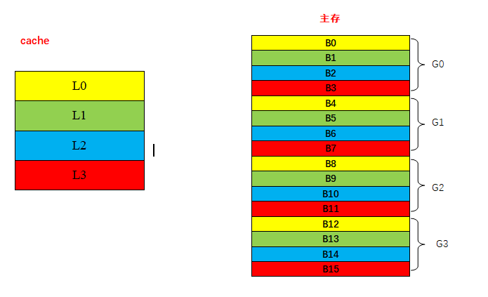
- 对主存进行分区: 16 ÷ 4 = 4 16 \div 4 = 4 16÷4=4,主存划分为 4 个分区,分区编号为 G0 ∼ G3 \text{G0} \sim \text{G3} G0∼G3,每个分区包含 4 个主存块。
- 分区内块重新编号:分区 G0 \text{G0} G0 内 B0、B1、B2、B3 \text{B0、B1、B2、B3} B0、B1、B2、B3 依次记为 b0、b1、b2、b3 \text{b0、b1、b2、b3} b0、b1、b2、b3;分区 G1 \text{G1} G1 内 B4、B5、B6、B7 \text{B4、B5、B6、B7} B4、B5、B6、B7 依次记为 b0、b1、b2、b3 \text{b0、b1、b2、b3} b0、b1、b2、b3,其余分区依照此规则顺延编号。
- 映射约束:分区内编号为 b0 \text{b0} b0 的主存块,仅可存入 cache 行 L0 \text{L0} L0;分区内编号为 b1 \text{b1} b1 的主存块,仅可存入 cache 行 L1 \text{L1} L1,以此类推。如上图所示,相同颜色的说明可以进行拷贝。
地址格式
- 主存地址格式:主存组号 + 组内块号 + 块内偏移地址
- cache 地址格式:cache 行号 + 行内偏移地址
- cache 标记
tag:对应主存块所属的主存组号
地址变换流程
CPU 向 cache 发送内存地址,硬件逻辑依据地址中的组内块号,确定当前主存块对应的目标 cache 行。
提取地址中的主存组号,与目标 cache 行的标记 tag 进行比对。
- 比对结果一致:判定为命中。
- 比对结果不一致:判定为未命中。
特性与应用场景
- 特性:硬件结构简单,实现成本低。主存块发生冲突的概率偏高,会降低数据读取效率。
- 适用场景:容量较大的 cache 系统,更多的 cache 行可降低块冲突出现的频次。
3. 组相联映射方式
基本规则
该方式结合直接映射与全相联映射的设计思路。将 cache 划分为若干组,主存块与 cache 组采用直接映射规则,同一 cache 组内部的行采用全相联映射规则。
划分规则:cache 的分组数量 等于 主存单个分区内的块数量。
相关定义
v v v 路组相联 cache:表示 cache 采用组相联映射,且每个 cache 组包含 v v v 行。 v v v 通常取 2、4、8、16 等数值。
示例设定
某主存-cache 体系中,cache 共 4 行,行编号为 L0 ∼ L3 \text{L0} \sim \text{L3} L0∼L3;主存共 16 块,块编号为 B0 ∼ B15 \text{B0} \sim \text{B15} B0∼B15,系统采用 2 路组相联映射。

- cache 分组:4 行 cache 划分为 2 个组,组编号为 G0 ∼ G1 \text{G0} \sim \text{G1} G0∼G1,每组包含 2 行。
- 主存分区:依照规则,主存单个分区包含 2 个块,16 个主存块共划分为 8 个分区,分区编号为 g0 ∼ g7 \text{g0} \sim \text{g7} g0∼g7。
- 分区内块重新编号:每个主存分区内的块依次编号为 b0、b1 \text{b0、b1} b0、b1。
- 映射约束:组内编号为 b0 \text{b0} b0 的主存块,可复制至 cache 组 G0 \text{G0} G0 内任意一行;组内编号为 b1 \text{b1} b1 的主存块,可复制至 cache 组 G1 \text{G1} G1 内任意一行。
地址格式
- 主存地址格式:主存组号 + 组内块号 + 块内偏移地址
- cache 地址格式:cache 组号 + 组内行号 + 行内偏移地址
- cache 标记
tag:主存组号
地址变换流程
CPU 向 cache 发送内存地址,硬件逻辑依据地址中的组内块号,确定当前主存块对应的目标 cache 组。
提取地址中的主存组号,与目标 cache 组内所有行的标记 tag 并行比对。
- 比对结果存在匹配项:判定为命中。
- 比对结果无匹配项:判定为未命中。
特性说明
该方式硬件实现难度适中,块冲突概率低于直接映射方式,系统命中率介于直接映射方式与全相联映射方式之间,在工程中得到广泛使用。
有关 cache 命中率的问题
发布时间:2017-12-07 14:40:24
参考资料:《计算机组成原理》(第五版) 白中英 等著
本文阐述 cache 命中率的计算方法、影响条件,结合实例说明未命中状态下主存访问时长的计算逻辑,分析 cache-主存存储系统的访问效率。
一、相关概念与计算公式
设定参数说明:
N c N_\text{c} Nc:程序运行过程中,cache 完成数据存取的总次数
N m N_\text{m} Nm:程序运行过程中,主存完成数据存取的总次数
h h h:cache 命中率
t c t_\text{c} tc:命中状态下,cache 的单次访问时长
t m t_\text{m} tm:未命中状态下,主存的单次访问时长
Cache-主存系统性能相关公式
1. Cache 命中率
h = N c N c + N m h=\frac{N_c}{N_c} \text{+}{N_m} h=NcNc+Nm
其中:
- h h h:Cache 命中率(Hit Rate)
- N c N_c Nc:Cache 命中时的访问次数
- N m N_m Nm:Cache 未命中时的主存访问次数
2. Cache-主存系统平均访问时间
t a = h t c + ( 1 − h ) t m t_a = h t_c + (1 - h) t_m ta=htc+(1−h)tm
其中:
- t c t_c tc:Cache 命中时的访问时间
- t m t_m tm:Cache 未命中时,访问主存的时间(包含访问 Cache 失败的时间)
3. 主存相对 Cache 的速度倍率
r = t m t c r = \frac{t_m}{t_c} r=tctm
4. 存储系统访问效率
e = t c t a = t c h t c + ( 1 − h ) t m = 1 h + ( 1 − h ) r = 1 r + ( 1 − r ) h e = \frac{t_c}{t_a} = \frac{t_c}{h t_c + (1 - h) t_m} = \frac{1}{h + (1 - h)r} = \frac{1}{r + (1 - r)h} e=tatc=htc+(1−h)tmtc=h+(1−h)r1=r+(1−r)h1
二、参数 t m t_\text{m} tm 的取值分析
依据教材定义, t m t_\text{m} tm 指代未命中状态下主存的整体访问时长,该参数不等同于主存自身的存储周期。结合实例进行说明:
实例条件
某计算机采用 cache-主存两级存储结构,cache 存储周期为 10 ns,主存存储周期为 50 ns。程序运行期间,cache 存取次数为 4800 次,主存存取次数为 200 次。硬件架构规定 cache 与主存不可并行访问,求解该存储系统的访问效率。
分析过程
系统出现未命中时,硬件会先完成一次 cache 访问,再执行主存访问。结合本题条件:
t m = 10 ns + 50 ns = 60 ns t_\text{m} = 10\ \text{ns} + 50\ \text{ns} = 60\ \text{ns} tm=10 ns+50 ns=60 ns
该取值方式基于习题场景推导,相关理论适配性仍可进一步研究。
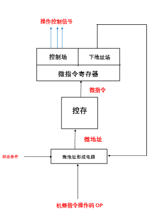
微程序控制器之微地址的形成
叫大顺但不顺 原创于 2017-12-11 12:09:44 发布
参考资料:《计算机组成原理》(第五版) 白中英 等著
执行当前微指令的过程中,需确定下一条微指令的地址,以此完成后续微指令的读取与执行,该逻辑与机器指令的寻址逻辑一致。
A、执行指令阶段首条微指令地址的形成
该地址也可定义为非取指微程序的微程序入口地址。
机器指令的操作码字段(OP 字段)经微地址形成部件处理,生成对应微程序的入口地址,并将该地址送入微地址寄存器。
非取指微程序的入口地址,可视为机器指令操作码对应的映射结果。
B、后继微指令地址的形成
后继微指令地址的生成包含两类实现形式:① 计数器方式 ;② 多路转移方式。
a、计数器方式
该方式的实现逻辑与程序计数器(PC)生成后继地址的方式相近。地址生成电路以微地址计数器(MPC 或 μ \mu μPC) 为核心,后继微地址由当前微地址叠加固定增量得到。
采用该方式时,微指令内部无需配置下地址字段;同时,顺序执行的多条微指令,必须连续存放于控制存储器的存储单元中。
b、多路转移方式(断定方式)
微指令内的顺序控制字段参与地址生成流程,地址转移逻辑依据字段信息,对微地址寄存器内部存储的地址数据进行修改。
Cache 地址映射、地址结构与行表项结构
一、三种地址映射方式相关要点
(一)全相联映射方式
- 优缺点
- 优势:主存块冲突概率低,Cache 空间利用率较高。
- 不足:硬件控制逻辑复杂,标记比对所用比较器电路设计与实现难度大,一般应用于小容量 Cache。
(二)直接映射方式
- 地址格式
- 主存地址:主存组号 + 组内块号 + 块内偏移地址
- Cache 地址:Cache 行号 + 行内偏移地址
- Cache 标记
tag:主存组号
(三)组相联映射方式
- 地址变换流程
- CPU 向 Cache 发送内存地址,硬件逻辑依据地址中的组内块号,确定主存块对应的目标 Cache 组。
- 提取地址内的主存组号,将其与目标 Cache 组内所有行的
tag并行比对。 - 存在匹配项则判定为命中;无匹配项则判定为未命中,系统转向主存读取数据。
二、Cache 地址结构与行表项结构
(一)Cache 地址结构
Cache 地址为硬件寻址依据,依靠地址字段的编号,完成目标 Cache 行、行内数据单元的定位。不同映射方式下,地址字段的划分形式各不相同。
(二)Cache 行(表项)存储结构
Cache 每一行对应一个独立表项,用于存放数据及各类控制标识,完整组成字段如下:
- 有效位:标识当前 Cache 行内数据是否有效。
- 标记位(tag):存储主存块的标识信息。主存块载入 Cache 行时,对应主存块标识会写入该字段;地址匹配阶段,硬件将主存地址中的块标识与标记位比对,以此判断该行是否存放目标主存块。
- 数据区:存储从主存拷贝的整块数据。
- 一致性维护位:用于维持 Cache 与主存的数据一致性,多应用于多级存储、多处理器架构场景。
- 替换控制位:配合替换算法记录行状态,Cache 空间不足时,辅助筛选待替换行。
区分说明
地址结构承担寻址定位 功能,用于选定待访问的 Cache 行;行表项结构承担状态记录与数据存储功能,标记位是行表项的组成字段,通过字段比对完成命中判断。
reference
-
What Your Computer Does While You Wait | 2008
https://manybutfinite.com/post/what-your-computer-does-while-you-wait/
-
Cache: a place for concealment and safekeeping | 2009
-
Anatomy of a Program in Memory | 2009
https://manybutfinite.com/post/anatomy-of-a-program-in-memory/
-
主存与 cache 间的地址映射_cache 地址格式-CSDN 博客
-
有关 cache 命中率的问题_cache 命中率与哪些因素有关-CSDN 博客
-
微程序控制器之微地址的形成_微地址形成部件-CSDN博客
-
...