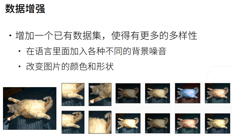
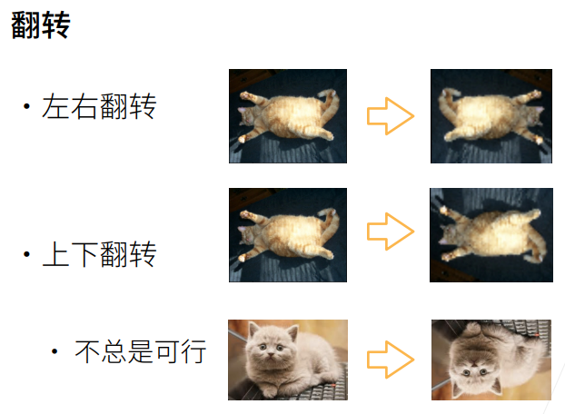
1. 数据增广

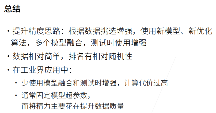
1. 总结

2. 数据增广-----代码
python
#让 matplotlib 绘制的图像直接内嵌显示在单元格输出下方,不会弹出独立图片窗口,是深度学习绘图标配。
%matplotlib inline
import torch                # 导入PyTorch深度学习框架,搭建、运行神经网络
import torchvision          # PyTorch配套视觉工具库,处理图像、数据集、预训练模型
from torch import nn        # 从torch单独导入神经网络模块(卷积层、全连接层、激活函数等)
from d2l import torch as d2l # 导入《动手学深度学习》配套工具包,封装了绘图、读图、训练辅助函数

d2l.set_figsize()   #调用 d2l 封装的接口,设置全局画布默认大小
img = d2l.Image.open('01_Data/02_cat.jpg') # 读取图片
d2l.plt.imshow(img) # 显示图片<matplotlib.image.AxesImage at 0x1d31b4730f0>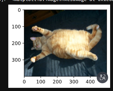
python
def apply(img, aug, num_rows=2, num_cols=4, scale=1.5): # 传入aug图片增广方法
    Y = [aug(img) for _ in range(num_rows * num_cols)] # 用aug方法对图片作用八次
    d2l.show_images(Y, num_rows, num_cols, scale=scale) # 生成结果用num_cols行,num_cols列展示
python
apply(img, torchvision.transforms.RandomHorizontalFlip()) # 水平随机翻转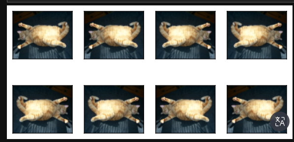
python
apply(img, torchvision.transforms.RandomVerticalFlip()) # 上下随机翻转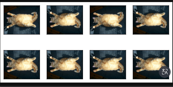
python
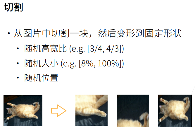
# 随机剪裁,剪裁后的大小为(200,200)
# (0.1,1)使得随即剪裁原始图片的10%到100%区域里的大小,ratio=(0.5,2)使得高宽比为2:1,下面是显示时显示的1:1
shape_aug = torchvision.transforms.RandomResizedCrop((200,200),scale=(0.1,1),ratio=(0.5,2))
apply(img,shape_aug)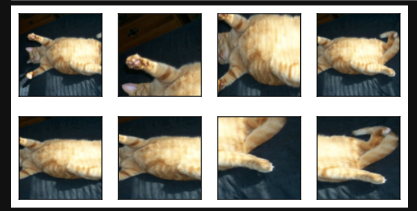
python
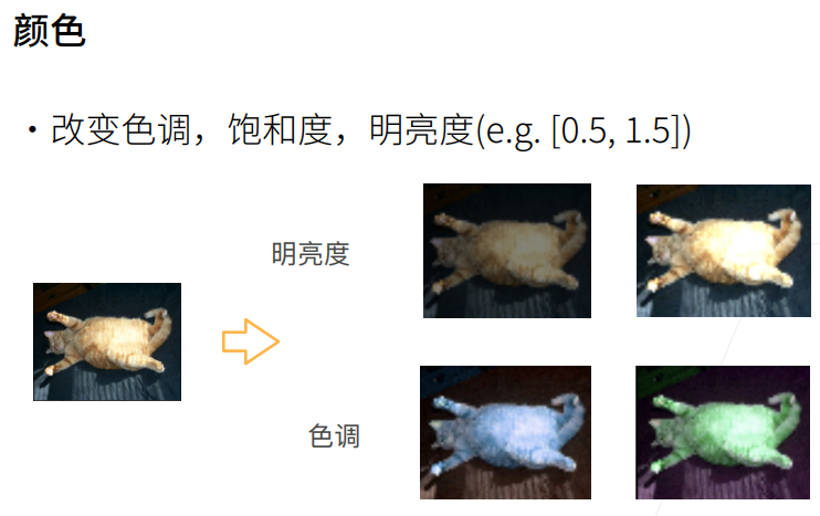
# 随即更改图像的亮度                          亮度          对比度       饱和度      色相
apply(img,torchvision.transforms.ColorJitter(brightness=0.5,contrast=0,saturation=0,hue=0)) 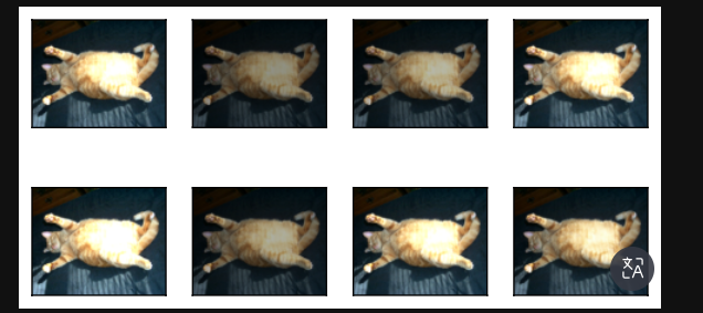
python
# 随即改变色调
apply(img,torchvision.transforms.ColorJitter(brightness=0,contrast=0,saturation=0,hue=0.5)) 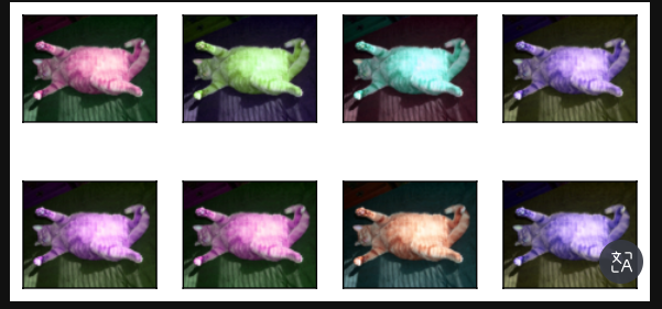
python
# 随机更改图像的亮度(brightness)、对比度(constrast)、饱和度(saturation)和色调(hue)
color_aug = torchvision.transforms.ColorJitter(brightness=0.5,contrast=0.5,saturation=0.5,hue=0.5)
apply(img,color_aug)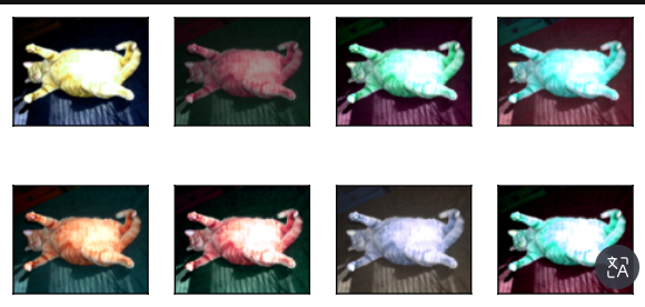
python
# 结合多种图像增广方法
# 先随即水平翻转,再做颜色增广,再做形状增广
augs = torchvision.transforms.Compose([torchvision.transforms.RandomHorizontalFlip(),color_aug,shape_aug])
apply(img,augs)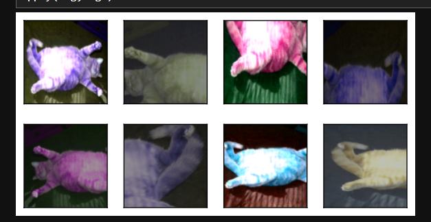
python
# 下载图片,并显示部分图片
all_images = torchvision.datasets.CIFAR10(train=True, root='01_Data/03_CIFAR10', download=True)
d2l.show_images([all_images[i][0] for i in range(32)], 4, 8, scale=0.8)Files already downloaded and verified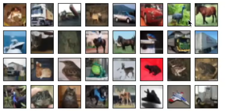
array([<AxesSubplot:>, <AxesSubplot:>, <AxesSubplot:>, <AxesSubplot:>,
       <AxesSubplot:>, <AxesSubplot:>, <AxesSubplot:>, <AxesSubplot:>,
       <AxesSubplot:>, <AxesSubplot:>, <AxesSubplot:>, <AxesSubplot:>,
       <AxesSubplot:>, <AxesSubplot:>, <AxesSubplot:>, <AxesSubplot:>,
       <AxesSubplot:>, <AxesSubplot:>, <AxesSubplot:>, <AxesSubplot:>,
       <AxesSubplot:>, <AxesSubplot:>, <AxesSubplot:>, <AxesSubplot:>,
       <AxesSubplot:>, <AxesSubplot:>, <AxesSubplot:>, <AxesSubplot:>,
       <AxesSubplot:>, <AxesSubplot:>, <AxesSubplot:>, <AxesSubplot:>],
      dtype=object)
python
# 只使用最简单的随机左右翻转
train_augs = torchvision.transforms.Compose([
    torchvision.transforms.RandomHorizontalFlip(),
    torchvision.transforms.ToTensor()])

test_augs = torchvision.transforms.Compose([
    torchvision.transforms.ToTensor()])
python
# 定义一个辅助函数,以便于读取图像和应用图像增广
def load_cifar10(is_train, augs, batch_size):
    dataset = torchvision.datasets.CIFAR10(root='01_Data/03_CIFAR10',train=is_train,
                                         transform=augs, download=True)
    dataloader = torch.utils.data.DataLoader(dataset,batch_size=batch_size,shuffle=is_train,
                                            num_workers = 0)
    return dataloader
python
# 定义一个函数,使用多GPU模式进行训练和评估
def train_batch_ch13(net, X, y, loss, trainer, devices):
    if isinstance(X, list):
        X = [x.to(devices[0]) for x in X] # 如果X是一个list,则把数据一个接一个都挪到devices[0]上
    else:
        X = X.to(devices[0]) # 如果X不是一个list,则把X挪到devices[0]上
    y = y.to(devices[0])
    net.train()
    trainer.zero_grad()
    pred = net(X)
    l = loss(pred, y)
    l.sum().backward()
    trainer.step()
    train_loss_sum = l.sum()
    train_acc_sum = d2l.accuracy(pred, y)
    return train_loss_sum, train_acc_sum

def train_ch13(net, train_iter, test_iter, loss, trainer, num_epochs, devices=d2l.try_all_gpus()):
    timer, num_batches = d2l.Timer(), len(train_iter)
    animator = d2l.Animator(xlabel='epoch',xlim=[1,num_epochs],ylim=[0,1],
                           legend=['train loss', 'train acc', 'test acc'])
    # nn.DataParallel使用多GPU
    net = nn.DataParallel(net, device_ids=devices).to(devices[0])
    for epoch in range(num_epochs):
        metric = d2l.Accumulator(4)
        for i, (features, labels) in enumerate(train_iter):
            timer.start()
            l, acc = train_batch_ch13(net,features,labels,loss,trainer,devices)
            metric.add(l,acc,labels.shape[0],labels.numel())
            timer.stop()
            if (i + 1) % (num_batches // 5) == 0 or i == num_batches -1:
                animator.add(
                    epoch + (i + 1) / num_batches,
                    (metric[0] / metric[2], metric[1] / metric[3], None))
        test_acc = d2l.evaluate_accuracy_gpu(net,test_iter)
        animator.add(epoch+1,(None,None,test_acc))
    print(f'loss {metric[0] / metric[2]:.3f}, train acc'
         f' {metric[1] / metric[3]:.3f}, test acc {test_acc:.3f}')
    print(f' {metric[2] * num_epochs / timer.sum():.1f} examples/sec on '
         f' {str(devices)}')
python
# 定义train_with_data_aug函数,使用图像增广来训练模型
batch_size, devices, net = 256, d2l.try_all_gpus(), d2l.resnet18(10,3)

def init_weights(m):
    if type(m) in [nn.Linear, nn.Conv2d]:
        nn.init.xavier_uniform_(m.weight)

net.apply(init_weights)

def train_with_data_aug(train_augs, test_augs, net, lr=0.001):
    train_iter = load_cifar10(True, train_augs, batch_size)
    test_iter = load_cifar10(False, test_augs, batch_size)
    loss = nn.CrossEntropyLoss(reduction="none")
    # Adam优化器算是一个比较平滑的SGD,它对学习率调参不是很敏感
    trainer = torch.optim.Adam(net.parameters(),lr=lr)
    train_ch13(net, train_iter, test_iter, loss, trainer, 10, devices)

train_with_data_aug(train_augs, test_augs, net)loss 0.166, train acc 0.942, test acc 0.832
1013.2 examples/sec on [device(type='cuda', index=0)]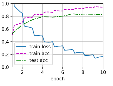
2. 微调

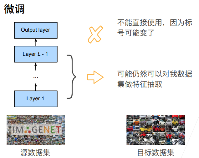
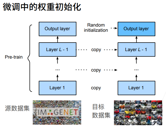
1. 总结

2. 微调---->代码
**目的:**自动下载热狗 / 非热狗二分类数据集,读取训练集、测试集,批量展示 8 张热狗图片 + 8 张非热狗图片
python
%matplotlib inline
import os                 #处理文件路径、文件夹
import torch
import torchvision         #深度学习框架、图像数据集工具
from torch import nn
from d2l import torch as d2l  #《动手学深度学习》配套工具库,自带数据集下载、绘图工具
python
#d2l.DATA_HUB 是一个字典,用来注册数据集信息:键名:hotdog(数据集名字)
#第一个值:数据集在线下载地址 hotdog.zip
#第二个值:文件校验码,用来判断文件有没有损坏、是否下载完整
d2l.DATA_HUB['hotdog'] = (d2l.DATA_URL + 'hotdog.zip','fba480ffa8aa7e0febbb511d181409f899b9baa5')
data_dir = d2l.download_extract('hotdog')#data_dir 变量保存解压后数据集根文件夹路径
# ImageFolder 读取文件夹式数据集
#train_imgs 是整个训练数据集对象,可以用下标取单条样本
train_imgs = torchvision.datasets.ImageFolder(os.path.join(data_dir,'train'))
test_imgs = torchvision.datasets.ImageFolder(os.path.join(data_dir,'test'))#
python
# 图片的大小和纵横比各有不同
#列表推导式循环 8 次,得到包含 8 张热狗图片的列表 hotdogs
hotdogs = [train_imgs[i][0] for i in range(8)]
print(train_imgs[0]) # 图片和标签,合为一个元组
print(train_imgs[0][0]) # 元组第一个元素为图片
not_hotdogs = [train_imgs[-i - 1][0] for i in range(8)]
d2l.show_images(hotdogs + not_hotdogs, 2, 8, scale=1.4)(<PIL.Image.Image image mode=RGB size=122x144 at 0x1F2CBDF9AC8>, 0)
<PIL.Image.Image image mode=RGB size=122x144 at 0x1F2CBDF9C18>array([<AxesSubplot:>, <AxesSubplot:>, <AxesSubplot:>, <AxesSubplot:>,
<AxesSubplot:>, <AxesSubplot:>, <AxesSubplot:>, <AxesSubplot:>,
<AxesSubplot:>, <AxesSubplot:>, <AxesSubplot:>, <AxesSubplot:>,
<AxesSubplot:>, <AxesSubplot:>, <AxesSubplot:>, <AxesSubplot:>],
dtype=object)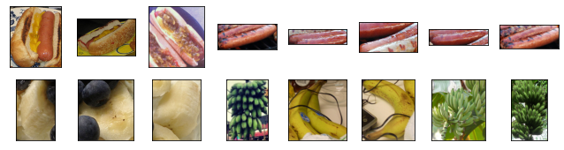
整体作用:分别定义训练集、测试集两套图像预处理流水线,在喂进神经网络前统一图片格式、做数据增强防过拟合,最后标准化像素值。
执行顺序从上到下:
- RandomResizedCrop(224) 随机裁剪 + 缩放:随机在原图抠一块区域,再缩放到
224×224正方形。 👉 数据增强:让模型学会关注物体不同局部位置,提升泛化能力。- RandomHorizontalFlip() 随机水平翻转:默认 50% 概率左右镜像翻转图片,另一半保持原图不变。 👉 扩充样本多样性,防止模型死记图片朝向。
- ToTensor() PIL 图片 → PyTorch 张量;同时把像素值从
0~255压缩到0~1。 通道顺序从(H,W,C)转为模型要求的(C,H,W)。- normalize 用上面定义的均值方差做标准化。
训练集 train_augs 测试集 test_augs 随机裁剪、随机翻转(数据增强) 居中裁剪、无任何随机操作 目的:扩充数据,防止过拟合 目的:统一输入尺寸,保证预测稳定可复现
python
# 数据增广
#Normalize(均值列表, 标准差列表)
normalize = torchvision.transforms.Normalize([0.485,0.456,0.406],
                                            [0.229,0.224,0.225]) # 按该均值、方差做归一化
#Compose = 把多个变换操作按顺序打包串联执行

train_augs = torchvision.transforms.Compose([
    torchvision.transforms.RandomResizedCrop(224),
    torchvision.transforms.RandomHorizontalFlip(),
    torchvision.transforms.ToTensor(),
    normalize ])

test_augs = torchvision.transforms.Compose([
    torchvision.transforms.Resize(256),
    torchvision.transforms.CenterCrop(224),
    torchvision.transforms.ToTensor(),
    normalize ])
含义拆解
torchvision.models.resnet18:调用 PyTorch 内置的 ResNet18 网络结构(18 层深度残差卷积神经网络,图像分类经典 backbone)pretrained=True
- 自动下载在超大 ImageNet 数据集上训练完成的权重参数
- 不是初始化随机参数,而是加载别人训练好、提取通用视觉特征的成熟权重
- 该技巧叫迁移学习:用大数据学到的通用视觉能力,适配你自己的热狗二分类小数据集,收敛更快、精度更高
ResNet18 前面一大堆卷积层、残差块,用来提取图片边缘、纹理、轮廓、物体高级特征; 末尾 fc = fully connected 全连接层,是整个网络最后的分类输出头。
python
# 定义和初始化模型
pretrained_net = torchvision.models.resnet18(pretrained=True) # 把模型和在ImageNet上定义好的参数拿过来
pretrained_net.fc # full connection全连接层,最后一层,查看最后一层的输入和输出结构 Linear(in_features=512, out_features=1000, bias=True)知识点讲解
- 前面卷积层是预训练好的成熟权重,不用重新初始化;
- 你刚刚新建替换的
fc层是随机初始值,需要合理初始化;xavier_uniform_是经典权重初始化方案: 让每一层输入、输出的方差尽量稳定,避免训练时梯度爆炸 / 梯度消失,收敛更快更稳;- 注意:只初始化了权重 weight,偏置 bias 默认 PyTorch 自带初始化,不用手动处理
python
finetune_net = torchvision.models.resnet18(pretrained=True)
finetune_net.fc = nn.Linear(finetune_net.fc.in_features,2) # 最后一层修改为输出类别数为2
nn.init.xavier_uniform_(finetune_net.fc.weight) # 只对最后一层的weight做随即初始化 Parameter containing:
tensor([[ 0.0004, -0.0395, -0.0163, ..., 0.0185, -0.0238, 0.0693],
[ 0.0307, 0.0278, 0.0082, ..., -0.0852, 0.0642, -0.0302]],
requires_grad=True)整体功能:针对迁移学习微调专门设计的训练函数,支持「主干小学习率、分类头大学习率」差异化训练,适配你的热狗二分类任务
参数说明:
net:你改造好的 ResNet18 模型finetune_net
learning_rate:基础学习率
batch_size=128:批次大小,每次喂入模型 128 张图
num_epochs=5:完整遍历整个数据集 5 轮
param_group=True:是否开启分组学习率(微调核心技巧)
ImageFolder:读取你热狗数据集,自动打标签
transform=train_augs / test_augs:自动套用前面写好的数据增强 + 归一化预处理
shuffle=True:训练集打乱顺序,防止模型记顺序作弊;测试集不需要打乱
python
# 微调座位
def train_fine_tuning(net, learning_rate, batch_size=128, num_epochs=5, param_group=True):
    train_iter = torch.utils.data.DataLoader(
        torchvision.datasets.ImageFolder(os.path.join(data_dir,'train'),transform=train_augs),
        batch_size = batch_size,shuffle=True)
    test_iter = torch.utils.data.DataLoader(
        torchvision.datasets.ImageFolder(os.path.join(data_dir,'test'),transform=test_augs),
        batch_size=batch_size)
#动检测电脑有没有 GPU,有就用 GPU 加速训练,没有自动切 CPU
    devices = d2l.try_all_gpus()
    loss = nn.CrossEntropyLoss(reduction="none")#交叉熵损失
    if param_group:          #params_lx:收集除最后全连接层 fc 以外所有卷积、残差层参数
        # 除了最后一层的learning rate外,用的是默认的learning rate
        # 最后一层的learning rate用的是十倍的learning rate
        params_lx = [
            param for name, param in net.named_parameters()
            if name not in ["fc.weight","fc.bias"] ]
        trainer = torch.optim.SGD([
            {'params': params_lx},
            {'params': net.fc.parameters(), 'lr': learning_rate * 10}],
            lr=learning_rate, weight_decay=0.001) #权重衰减(L2 正则),抑制过拟合
   #全部参数共用同一个学习率,适合全程从头大幅度训练,微调场景一般不用。
     else:
        trainer = torch.optim.SGD(net.parameters(),lr=learning_rate,weight_decay=0.001)
#调用 d2l 封装好的第 13 章训练循环:自动完成前向传播、反向传播、参数更新、打印训练 / 测试准确率、损失变化
    d2l.train_ch13(net, train_iter, test_iter, loss, trainer, num_epochs,devices)
python
# 使用较小的学习率
train_fine_tuning(finetune_net,5e-5)loss 0.163, train acc 0.932, test acc 0.935
265.9 examples/sec on [device(type='cuda', index=0)]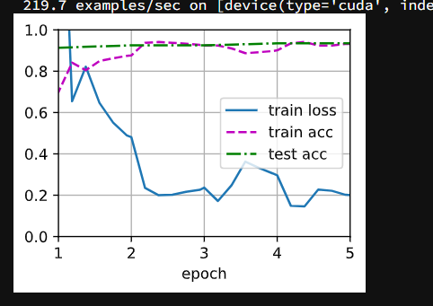
python
# 为了进行比较,所有模型参数初始化为随机值
scratch_net = torchvision.models.resnet18() # 这里没有pretrained=True,没有拿预训练的参数
scratch_net.fc = nn.Linear(scratch_net.fc.in_features,2)
train_fine_tuning(scratch_net,5e-4,param_group=False) # param_group=False使得所有层的参数都为默认的学习率 loss 0.349, train acc 0.847, test acc 0.806
422.1 examples/sec on [device(type='cuda', index=0)]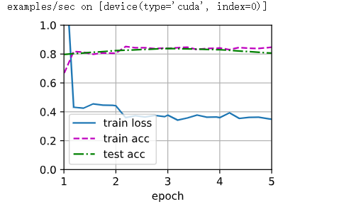
为什么微调要用「两头不同学习率」?💡
- 前面卷积层:已经学会识别边缘、纹理、物体轮廓等通用视觉知识,只需要小幅修正适配新数据集,学习率必须很小,步子大容易冲乱原有优质权重
- 最后 fc 层:是你全新初始化的,完全不认识热狗分类,需要更快收敛,所以设置10 倍更大学习率加速学习
3. 实战Kaggle比赛图像分类CIFAR10
① 比赛的网址是 Checking your browser - reCAPTCHA
python
import collections
import math
import os
import shutil
import pandas as pd
import torch
import torchvision
from torch import nn
from d2l import torch as d2l
python
# 我们提供包含前1000个训练图像和5个随即测试图像的数据集的小规模样本
# cifar10_tiny是cifar10中每一个类把前面一千个训练图片拿出来,测试是每一个类挑五个图片
d2l.DATA_HUB['cifar10_tiny'] = (d2l.DATA_URL + 'kaggle_cifar10_tiny.zip',
                               '2068874e4b9a9f0fb07ebe0ad2b29754449ccacd')
demo = True

if demo:
    data_dir = d2l.download_extract('cifar10_tiny')
else:
    data_dir = '../data/cifar-10'
python
# 整理数据集
def read_csv_labels(fname):
    """读取 'fname' 来给标签字典返回一个文件名。"""
    with open(fname, 'r') as f:
        lines = f.readlines()[1:] # 一行一行读进来,每一行为列表中一个元素
    tokens = [l.rstrip().split(',') for l in lines] # 遍历列表每一个元素,切分
    return dict(((name, label) for name, label in tokens))

labels = read_csv_labels(os.path.join(data_dir,'trainLabels.csv'))
labels{'1': 'frog',
'2': 'truck',
'3': 'truck',
'4': 'deer',
'5': 'automobile',
'6': 'automobile',
'7': 'bird',
'8': 'horse',
'9': 'ship',
'10': 'cat',
'11': 'deer',
'12': 'horse',
'13': 'horse',
'14': 'bird',
'15': 'truck',
'16': 'truck',
'17': 'truck',
'18': 'cat',
'19': 'bird',
'20': 'frog',
'21': 'deer',
'22': 'cat',
'23': 'frog',
'24': 'frog',
'25': 'bird',
'26': 'frog',
'27': 'cat',
'28': 'dog',
'29': 'deer',
'30': 'airplane',
'31': 'airplane',
'32': 'truck',
'33': 'automobile',
'34': 'cat',
'35': 'deer',
'36': 'airplane',
'37': 'cat',
'38': 'horse',
'39': 'cat',
'40': 'cat',
'41': 'dog',
'42': 'bird',
'43': 'bird',
'44': 'horse',
'45': 'automobile',
'46': 'automobile',
'47': 'automobile',
'48': 'bird',
'49': 'bird',
'50': 'airplane',
'51': 'truck',
'52': 'dog',
'53': 'horse',
'54': 'truck',
'55': 'bird',
'56': 'bird',
'57': 'dog',
'58': 'bird',
'59': 'deer',
'60': 'cat',
'61': 'automobile',
'62': 'automobile',
'63': 'ship',
'64': 'bird',
'65': 'automobile',
'66': 'automobile',
'67': 'deer',
'68': 'truck',
'69': 'horse',
'70': 'ship',
'71': 'dog',
'72': 'truck',
'73': 'frog',
'74': 'horse',
'75': 'cat',
'76': 'automobile',
'77': 'truck',
'78': 'airplane',
'79': 'cat',
'80': 'automobile',
'81': 'cat',
'82': 'dog',
'83': 'deer',
'84': 'dog',
'85': 'horse',
'86': 'horse',
'87': 'deer',
'88': 'horse',
'89': 'truck',
'90': 'deer',
'91': 'bird',
'92': 'cat',
'93': 'ship',
'94': 'airplane',
'95': 'automobile',
'96': 'frog',
'97': 'automobile',
'98': 'automobile',
'99': 'deer',
'100': 'automobile',
'101': 'ship',
'102': 'cat',
'103': 'truck',
'104': 'frog',
'105': 'frog',
'106': 'automobile',
'107': 'ship',
'108': 'dog',
'109': 'bird',
'110': 'truck',
'111': 'truck',
'112': 'ship',
'113': 'automobile',
'114': 'horse',
'115': 'horse',
'116': 'airplane',
'117': 'airplane',
'118': 'frog',
'119': 'truck',
'120': 'automobile',
'121': 'bird',
'122': 'bird',
'123': 'truck',
'124': 'bird',
'125': 'frog',
'126': 'frog',
'127': 'automobile',
'128': 'truck',
'129': 'dog',
'130': 'airplane',
'131': 'deer',
'132': 'horse',
'133': 'frog',
'134': 'horse',
'135': 'automobile',
'136': 'ship',
'137': 'automobile',
'138': 'automobile',
'139': 'bird',
'140': 'ship',
'141': 'automobile',
'142': 'cat',
'143': 'cat',
'144': 'frog',
'145': 'bird',
'146': 'deer',
'147': 'truck',
'148': 'truck',
'149': 'dog',
'150': 'deer',
'151': 'cat',
'152': 'frog',
'153': 'horse',
'154': 'deer',
'155': 'frog',
'156': 'ship',
'157': 'dog',
'158': 'dog',
'159': 'deer',
'160': 'cat',
'161': 'automobile',
'162': 'ship',
'163': 'deer',
'164': 'horse',
'165': 'frog',
'166': 'airplane',
'167': 'truck',
'168': 'dog',
'169': 'automobile',
'170': 'cat',
'171': 'ship',
'172': 'bird',
'173': 'horse',
'174': 'dog',
'175': 'cat',
'176': 'deer',
'177': 'automobile',
'178': 'dog',
'179': 'horse',
'180': 'airplane',
'181': 'deer',
'182': 'horse',
'183': 'dog',
'184': 'dog',
'185': 'automobile',
'186': 'airplane',
'187': 'truck',
'188': 'frog',
'189': 'truck',
'190': 'airplane',
'191': 'ship',
'192': 'horse',
'193': 'ship',
'194': 'ship',
'195': 'bird',
'196': 'dog',
'197': 'bird',
'198': 'cat',
'199': 'dog',
'200': 'airplane',
'201': 'frog',
'202': 'automobile',
'203': 'truck',
'204': 'cat',
'205': 'frog',
'206': 'truck',
'207': 'automobile',
'208': 'cat',
'209': 'truck',
'210': 'frog',
'211': 'frog',
'212': 'horse',
'213': 'automobile',
'214': 'airplane',
'215': 'truck',
'216': 'dog',
'217': 'ship',
'218': 'dog',
'219': 'bird',
'220': 'truck',
'221': 'airplane',
'222': 'ship',
'223': 'ship',
'224': 'airplane',
'225': 'frog',
'226': 'truck',
'227': 'automobile',
'228': 'automobile',
'229': 'frog',
'230': 'cat',
'231': 'horse',
'232': 'frog',
'233': 'frog',
'234': 'airplane',
'235': 'frog',
'236': 'frog',
'237': 'automobile',
'238': 'horse',
'239': 'automobile',
'240': 'dog',
'241': 'ship',
'242': 'cat',
'243': 'frog',
'244': 'frog',
'245': 'ship',
'246': 'frog',
'247': 'ship',
'248': 'deer',
'249': 'frog',
'250': 'frog',
'251': 'automobile',
'252': 'cat',
'253': 'ship',
'254': 'cat',
'255': 'deer',
'256': 'automobile',
'257': 'horse',
'258': 'automobile',
'259': 'cat',
'260': 'ship',
'261': 'dog',
'262': 'automobile',
'263': 'automobile',
'264': 'deer',
'265': 'airplane',
'266': 'truck',
'267': 'cat',
'268': 'horse',
'269': 'deer',
'270': 'truck',
'271': 'truck',
'272': 'bird',
'273': 'deer',
'274': 'truck',
'275': 'truck',
'276': 'automobile',
'277': 'airplane',
'278': 'dog',
'279': 'truck',
'280': 'airplane',
'281': 'ship',
'282': 'bird',
'283': 'automobile',
'284': 'bird',
'285': 'airplane',
'286': 'dog',
'287': 'frog',
'288': 'cat',
'289': 'bird',
'290': 'horse',
'291': 'ship',
'292': 'ship',
'293': 'frog',
'294': 'airplane',
'295': 'horse',
'296': 'truck',
'297': 'deer',
'298': 'dog',
'299': 'frog',
'300': 'deer',
'301': 'bird',
'302': 'automobile',
'303': 'automobile',
'304': 'bird',
'305': 'automobile',
'306': 'dog',
'307': 'truck',
'308': 'truck',
'309': 'airplane',
'310': 'ship',
'311': 'deer',
'312': 'automobile',
'313': 'automobile',
'314': 'frog',
'315': 'cat',
'316': 'cat',
'317': 'truck',
'318': 'airplane',
'319': 'horse',
'320': 'truck',
'321': 'horse',
'322': 'horse',
'323': 'truck',
'324': 'automobile',
'325': 'dog',
'326': 'automobile',
'327': 'frog',
'328': 'frog',
'329': 'ship',
'330': 'horse',
'331': 'automobile',
'332': 'cat',
'333': 'airplane',
'334': 'cat',
'335': 'cat',
'336': 'bird',
'337': 'deer',
'338': 'dog',
'339': 'horse',
'340': 'dog',
'341': 'truck',
'342': 'airplane',
'343': 'cat',
'344': 'deer',
'345': 'airplane',
'346': 'deer',
'347': 'deer',
'348': 'frog',
'349': 'airplane',
'350': 'airplane',
'351': 'frog',
'352': 'frog',
'353': 'airplane',
'354': 'ship',
'355': 'automobile',
'356': 'frog',
'357': 'bird',
'358': 'truck',
'359': 'bird',
'360': 'dog',
'361': 'truck',
'362': 'frog',
'363': 'horse',
'364': 'deer',
'365': 'automobile',
'366': 'ship',
'367': 'horse',
'368': 'cat',
'369': 'frog',
'370': 'truck',
'371': 'cat',
'372': 'airplane',
'373': 'deer',
'374': 'airplane',
'375': 'dog',
'376': 'automobile',
'377': 'airplane',
'378': 'cat',
'379': 'deer',
'380': 'ship',
'381': 'dog',
'382': 'deer',
'383': 'horse',
'384': 'bird',
'385': 'cat',
'386': 'truck',
'387': 'horse',
'388': 'frog',
'389': 'horse',
'390': 'automobile',
'391': 'deer',
'392': 'horse',
'393': 'airplane',
'394': 'automobile',
'395': 'horse',
'396': 'cat',
'397': 'automobile',
'398': 'ship',
'399': 'deer',
'400': 'deer',
'401': 'bird',
'402': 'airplane',
'403': 'bird',
'404': 'bird',
'405': 'airplane',
'406': 'airplane',
'407': 'truck',
'408': 'airplane',
'409': 'truck',
'410': 'frog',
'411': 'ship',
'412': 'bird',
'413': 'horse',
'414': 'horse',
'415': 'deer',
'416': 'airplane',
'417': 'cat',
'418': 'airplane',
'419': 'ship',
'420': 'truck',
'421': 'deer',
'422': 'bird',
'423': 'horse',
'424': 'bird',
'425': 'dog',
'426': 'bird',
'427': 'dog',
'428': 'automobile',
'429': 'truck',
'430': 'deer',
'431': 'ship',
'432': 'dog',
'433': 'automobile',
'434': 'horse',
'435': 'deer',
'436': 'deer',
'437': 'airplane',
'438': 'frog',
'439': 'truck',
'440': 'airplane',
'441': 'horse',
'442': 'ship',
'443': 'ship',
'444': 'truck',
'445': 'truck',
'446': 'cat',
'447': 'cat',
'448': 'deer',
'449': 'airplane',
'450': 'deer',
'451': 'dog',
'452': 'frog',
'453': 'frog',
'454': 'airplane',
'455': 'automobile',
'456': 'airplane',
'457': 'ship',
'458': 'airplane',
'459': 'deer',
'460': 'ship',
'461': 'ship',
'462': 'automobile',
'463': 'dog',
'464': 'bird',
'465': 'frog',
'466': 'ship',
'467': 'automobile',
'468': 'airplane',
'469': 'airplane',
'470': 'horse',
'471': 'horse',
'472': 'dog',
'473': 'truck',
'474': 'frog',
'475': 'bird',
'476': 'ship',
'477': 'cat',
'478': 'deer',
'479': 'horse',
'480': 'cat',
'481': 'truck',
'482': 'airplane',
'483': 'automobile',
'484': 'bird',
'485': 'deer',
'486': 'ship',
'487': 'automobile',
'488': 'ship',
'489': 'frog',
'490': 'deer',
'491': 'deer',
'492': 'dog',
'493': 'horse',
'494': 'automobile',
'495': 'cat',
'496': 'truck',
'497': 'ship',
'498': 'airplane',
'499': 'automobile',
'500': 'horse',
'501': 'dog',
'502': 'ship',
'503': 'bird',
'504': 'ship',
'505': 'airplane',
'506': 'deer',
'507': 'automobile',
'508': 'ship',
'509': 'truck',
'510': 'ship',
'511': 'bird',
'512': 'truck',
'513': 'truck',
'514': 'bird',
'515': 'horse',
'516': 'dog',
'517': 'horse',
'518': 'cat',
'519': 'ship',
'520': 'ship',
'521': 'deer',
'522': 'deer',
'523': 'bird',
'524': 'horse',
'525': 'automobile',
'526': 'frog',
'527': 'deer',
'528': 'airplane',
'529': 'deer',
'530': 'frog',
'531': 'truck',
'532': 'horse',
'533': 'frog',
'534': 'bird',
'535': 'dog',
'536': 'dog',
'537': 'automobile',
'538': 'horse',
'539': 'bird',
'540': 'bird',
'541': 'bird',
'542': 'truck',
'543': 'dog',
'544': 'deer',
'545': 'bird',
'546': 'horse',
'547': 'ship',
'548': 'automobile',
'549': 'cat',
'550': 'deer',
'551': 'cat',
'552': 'horse',
'553': 'frog',
'554': 'truck',
'555': 'ship',
'556': 'airplane',
'557': 'frog',
'558': 'airplane',
'559': 'bird',
'560': 'bird',
'561': 'bird',
'562': 'automobile',
'563': 'ship',
'564': 'deer',
'565': 'airplane',
'566': 'automobile',
'567': 'ship',
'568': 'ship',
'569': 'automobile',
'570': 'dog',
'571': 'horse',
'572': 'frog',
'573': 'deer',
'574': 'dog',
'575': 'ship',
'576': 'horse',
'577': 'automobile',
'578': 'truck',
'579': 'automobile',
'580': 'truck',
'581': 'ship',
'582': 'deer',
'583': 'horse',
'584': 'cat',
'585': 'ship',
'586': 'ship',
'587': 'bird',
'588': 'frog',
'589': 'frog',
'590': 'horse',
'591': 'automobile',
'592': 'frog',
'593': 'ship',
'594': 'automobile',
'595': 'truck',
'596': 'horse',
'597': 'ship',
'598': 'cat',
'599': 'airplane',
'600': 'automobile',
'601': 'airplane',
'602': 'ship',
'603': 'ship',
'604': 'cat',
'605': 'airplane',
'606': 'airplane',
'607': 'automobile',
'608': 'dog',
'609': 'airplane',
'610': 'ship',
'611': 'ship',
'612': 'horse',
'613': 'truck',
'614': 'truck',
'615': 'airplane',
'616': 'truck',
'617': 'deer',
'618': 'automobile',
'619': 'cat',
'620': 'frog',
'621': 'frog',
'622': 'deer',
'623': 'deer',
'624': 'horse',
'625': 'dog',
'626': 'frog',
'627': 'airplane',
'628': 'ship',
'629': 'airplane',
'630': 'cat',
'631': 'bird',
'632': 'ship',
'633': 'deer',
'634': 'frog',
'635': 'truck',
'636': 'truck',
'637': 'horse',
'638': 'airplane',
'639': 'cat',
'640': 'cat',
'641': 'frog',
'642': 'horse',
'643': 'deer',
'644': 'truck',
'645': 'automobile',
'646': 'frog',
'647': 'bird',
'648': 'horse',
'649': 'bird',
'650': 'bird',
'651': 'airplane',
'652': 'frog',
'653': 'horse',
'654': 'dog',
'655': 'horse',
'656': 'frog',
'657': 'ship',
'658': 'truck',
'659': 'airplane',
'660': 'truck',
'661': 'deer',
'662': 'deer',
'663': 'horse',
'664': 'airplane',
'665': 'truck',
'666': 'deer',
'667': 'truck',
'668': 'frog',
'669': 'truck',
'670': 'deer',
'671': 'dog',
'672': 'horse',
'673': 'truck',
'674': 'bird',
'675': 'deer',
'676': 'dog',
'677': 'automobile',
'678': 'deer',
'679': 'cat',
'680': 'truck',
'681': 'frog',
'682': 'dog',
'683': 'frog',
'684': 'truck',
'685': 'cat',
'686': 'cat',
'687': 'dog',
'688': 'airplane',
'689': 'horse',
'690': 'bird',
'691': 'automobile',
'692': 'cat',
'693': 'frog',
'694': 'deer',
'695': 'airplane',
'696': 'airplane',
'697': 'bird',
'698': 'dog',
'699': 'airplane',
'700': 'automobile',
'701': 'airplane',
'702': 'bird',
'703': 'cat',
'704': 'truck',
'705': 'ship',
'706': 'deer',
'707': 'truck',
'708': 'ship',
'709': 'airplane',
'710': 'bird',
'711': 'frog',
'712': 'deer',
'713': 'deer',
'714': 'airplane',
'715': 'automobile',
'716': 'ship',
'717': 'ship',
'718': 'cat',
'719': 'frog',
'720': 'truck',
'721': 'frog',
'722': 'frog',
'723': 'horse',
'724': 'ship',
'725': 'bird',
'726': 'deer',
'727': 'dog',
'728': 'horse',
'729': 'frog',
'730': 'dog',
'731': 'cat',
'732': 'airplane',
'733': 'dog',
'734': 'airplane',
'735': 'dog',
'736': 'airplane',
'737': 'ship',
'738': 'bird',
'739': 'frog',
'740': 'horse',
'741': 'cat',
'742': 'ship',
'743': 'bird',
'744': 'automobile',
'745': 'horse',
'746': 'frog',
'747': 'horse',
'748': 'automobile',
'749': 'airplane',
'750': 'truck',
'751': 'dog',
'752': 'dog',
'753': 'airplane',
'754': 'automobile',
'755': 'horse',
'756': 'frog',
'757': 'truck',
'758': 'airplane',
'759': 'deer',
'760': 'horse',
'761': 'horse',
'762': 'automobile',
'763': 'dog',
'764': 'truck',
'765': 'deer',
'766': 'airplane',
'767': 'ship',
'768': 'dog',
'769': 'truck',
'770': 'truck',
'771': 'frog',
'772': 'horse',
'773': 'automobile',
'774': 'ship',
'775': 'cat',
'776': 'bird',
'777': 'cat',
'778': 'ship',
'779': 'bird',
'780': 'bird',
'781': 'deer',
'782': 'frog',
'783': 'airplane',
'784': 'airplane',
'785': 'dog',
'786': 'cat',
'787': 'ship',
'788': 'bird',
'789': 'cat',
'790': 'horse',
'791': 'bird',
'792': 'truck',
'793': 'cat',
'794': 'ship',
'795': 'horse',
'796': 'ship',
'797': 'bird',
'798': 'horse',
'799': 'truck',
'800': 'airplane',
'801': 'bird',
'802': 'cat',
'803': 'bird',
'804': 'bird',
'805': 'bird',
'806': 'cat',
'807': 'cat',
'808': 'frog',
'809': 'bird',
'810': 'cat',
'811': 'bird',
'812': 'ship',
'813': 'airplane',
'814': 'dog',
'815': 'dog',
'816': 'automobile',
'817': 'deer',
'818': 'dog',
'819': 'frog',
'820': 'frog',
'821': 'bird',
'822': 'horse',
'823': 'airplane',
'824': 'automobile',
'825': 'horse',
'826': 'horse',
'827': 'ship',
'828': 'bird',
'829': 'truck',
'830': 'bird',
'831': 'bird',
'832': 'deer',
'833': 'bird',
'834': 'automobile',
'835': 'automobile',
'836': 'automobile',
'837': 'frog',
'838': 'frog',
'839': 'frog',
'840': 'dog',
'841': 'automobile',
'842': 'automobile',
'843': 'horse',
'844': 'airplane',
'845': 'deer',
'846': 'cat',
'847': 'cat',
'848': 'horse',
'849': 'automobile',
'850': 'bird',
'851': 'cat',
'852': 'dog',
'853': 'dog',
'854': 'dog',
'855': 'frog',
'856': 'automobile',
'857': 'deer',
'858': 'cat',
'859': 'horse',
'860': 'ship',
'861': 'ship',
'862': 'cat',
'863': 'frog',
'864': 'frog',
'865': 'bird',
'866': 'cat',
'867': 'airplane',
'868': 'truck',
'869': 'deer',
'870': 'cat',
'871': 'ship',
'872': 'airplane',
'873': 'airplane',
'874': 'automobile',
'875': 'automobile',
'876': 'dog',
'877': 'deer',
'878': 'truck',
'879': 'cat',
'880': 'automobile',
'881': 'ship',
'882': 'truck',
'883': 'cat',
'884': 'truck',
'885': 'truck',
'886': 'bird',
'887': 'truck',
'888': 'deer',
'889': 'ship',
'890': 'bird',
'891': 'truck',
'892': 'ship',
'893': 'ship',
'894': 'automobile',
'895': 'dog',
'896': 'cat',
'897': 'frog',
'898': 'ship',
'899': 'horse',
'900': 'frog',
'901': 'truck',
'902': 'ship',
'903': 'airplane',
'904': 'frog',
'905': 'deer',
'906': 'airplane',
'907': 'airplane',
'908': 'bird',
'909': 'dog',
'910': 'ship',
'911': 'bird',
'912': 'airplane',
'913': 'bird',
'914': 'horse',
'915': 'frog',
'916': 'truck',
'917': 'horse',
'918': 'automobile',
'919': 'dog',
'920': 'dog',
'921': 'frog',
'922': 'frog',
'923': 'cat',
'924': 'frog',
'925': 'bird',
'926': 'deer',
'927': 'horse',
'928': 'airplane',
'929': 'dog',
'930': 'frog',
'931': 'deer',
'932': 'frog',
'933': 'dog',
'934': 'bird',
'935': 'deer',
'936': 'frog',
'937': 'automobile',
'938': 'frog',
'939': 'airplane',
'940': 'deer',
'941': 'airplane',
'942': 'cat',
'943': 'automobile',
'944': 'ship',
'945': 'dog',
'946': 'deer',
'947': 'deer',
'948': 'automobile',
'949': 'horse',
'950': 'cat',
'951': 'truck',
'952': 'deer',
'953': 'horse',
'954': 'truck',
'955': 'horse',
'956': 'cat',
'957': 'horse',
'958': 'bird',
'959': 'ship',
'960': 'deer',
'961': 'frog',
'962': 'frog',
'963': 'automobile',
'964': 'bird',
'965': 'truck',
'966': 'airplane',
'967': 'deer',
'968': 'ship',
'969': 'horse',
'970': 'cat',
'971': 'truck',
'972': 'ship',
'973': 'horse',
'974': 'horse',
'975': 'airplane',
'976': 'bird',
'977': 'deer',
'978': 'automobile',
'979': 'automobile',
'980': 'deer',
'981': 'automobile',
'982': 'dog',
'983': 'deer',
'984': 'airplane',
'985': 'dog',
'986': 'frog',
'987': 'bird',
'988': 'ship',
'989': 'dog',
'990': 'airplane',
'991': 'bird',
'992': 'automobile',
'993': 'cat',
'994': 'dog',
'995': 'horse',
'996': 'cat',
'997': 'dog',
'998': 'automobile',
'999': 'cat',
'1000': 'dog'}
python
# 将验证集从原始的训练集中拆分出来
# train文件夹下有所有train的图片,test文件夹下有所有test图片
# 把train文件夹下所有类的图片创建一个类名文件夹,然后搬到对应文件夹下
def copyfile(filename, target_dir):
    """将文件复制到目标目录"""
    os.makedirs(target_dir, exist_ok=True)
    shutil.copy(filename, target_dir)
python
def reorg_train_valid(data_dir, labels, valid_ratio):
    n = collections.Counter(labels.values()).most_common()[-1][1]
    n_valid_per_label = max(1,math.floor(n * valid_ratio))
    label_count = {}
    for train_file in os.listdir(os.path.join(data_dir,'train')):
        label = labels[train_file.split('.')[0]]
        fname = os.path.join(data_dir,'train',train_file)
        copyfile(fname,os.path.join(data_dir,'train_valid_test','train_valid',label))
        if label not in label_count or label_count[label] < n_valid_per_label:
            copyfile(fname,os.path.join(data_dir,'train_valid_test','valid',label))
            label_count[label] = label_count.get(label,0) + 1
        else:
            copyfile(fname,os.path.join(data_dir,'train_valid_test','train',label))
    return n_valid_per_label
python
# 在预测期间整理测试集,以方便读取
def reorg_test(data_dir):
    for test_file in os.listdir(os.path.join(data_dir,'test')):
        copyfile(os.path.join(data_dir,'test',test_file),
                os.path.join(data_dir,'train_valid_test','test','unknown')) # unknown为 test文件夹里面的一个文件夹
python
# 调用前面定义的函数,前面只是定义函数,这里是调用
def reorg_cifar10_data(data_dir,valid_ratio):
    labels = read_csv_labels(os.path.join(data_dir,'trainLabels.csv'))
    reorg_train_valid(data_dir,labels,valid_ratio)
    reorg_test(data_dir)

batch_size = 32 if demo else 128
valid_ratio = 0.1 # train 数据里面百分之九十用来训练,剩下百分之十用来验证
reorg_cifar10_data(data_dir, valid_ratio)
python
# 图像增广
transform_train = torchvision.transforms.Compose([
    torchvision.transforms.Resize(40),
    torchvision.transforms.RandomResizedCrop(32,scale=(0.64,1.0),ratio=(1.0,1.0)),
    torchvision.transforms.RandomHorizontalFlip(),
    torchvision.transforms.ToTensor(),
    torchvision.transforms.Normalize([0.4914,0.4822,0.4465],
                                   [0.2023,0.1994,0.2010]) ])

transform_test = torchvision.transforms.Compose([
    torchvision.transforms.ToTensor(),
    torchvision.transforms.Normalize([0.4914,0.4822,0.4465],
                                    [0.2023,0.1994,0.2010]) ])
python
# 读取由原始图像组成的数据集
train_ds, train_valid_ds = [
    torchvision.datasets.ImageFolder(
        os.path.join(data_dir,'train_valid_test',folder),
        transform=transform_train) for folder in ['train','train_valid'] ]

valid_ds, test_ds = [
    torchvision.datasets.ImageFolder(
        os.path.join(data_dir,'train_valid_test',folder),
        transform=transform_test) for folder in ['valid','test'] ]
python
# 指定上面定义的所有图像增广操作
train_iter, train_valid_iter = [
    torch.utils.data.DataLoader(dataset,batch_size,shuffle=True,drop_last=True)
    for dataset in (train_ds, train_valid_ds) ]

valid_iter = torch.utils.data.DataLoader(valid_ds,batch_size,shuffle=False,drop_last=True)
test_iter = torch.utils.data.DataLoader(test_ds,batch_size,shuffle=False,drop_last=False)
python
# 模型
def get_net():
    num_classes = 10
    net = d2l.resnet18(num_classes,3) # 3表示数值三通道,彩色图片
    return net

loss = nn.CrossEntropyLoss(reduction="none") # reduction="none" 表示不要把loss加起来sum
python
# 训练函数
def train(net, train_iter, valid_iter, num_epoch, lr, wd, devices, lr_period, lr_decay):  # 每隔一段时间的lr_period把学习率lr_decay降低点
    trainer = torch.optim.SGD(net.parameters(),lr=lr,momentum=0.9,weight_decay=wd)
    scheduler = torch.optim.lr_scheduler.StepLR(trainer, lr_period, lr_decay)
    num_batches, timer = len(train_iter), d2l.Timer()
    legend = ['train loss','train acc']
    if valid_iter is not None:
        legend.append('valid acc')
    animator = d2l.Animator(xlabel='epoch',xlim=[1,num_epochs],legend=legend)
    net = nn.DataParallel(net,device_ids=devices).to(devices[0])
    for epoch in range(num_epochs):
        net.train()
        metric = d2l.Accumulator(3)
        for i,(features,labels) in enumerate(train_iter):
            timer.start()
            l, acc = d2l.train_batch_ch13(net,features,labels,loss,trainer,devices)
            metric.add(l,acc,labels.shape[0])
            timer.stop()
            if (i+1) % (num_batches // 5) == 0 or i == num_batches -1:
                animator.add(epoch + (i + 1) / num_batches, (metric[0]/metric[2], metric[1]/metric[2],None))
        if valid_iter is not None:
            valid_acc = d2l.evaluate_accuracy_gpu(net,valid_iter)
            animator.add(epoch+1,(None,None,valid_acc))
        scheduler.step()
    measures = (f'train loss {metric[0] / metric[2]:.3f},'
               f'train acc {metric[1] / metric[2]:.3f}')
    if valid_iter is not None:
        measures += f', valid acc {valid_acc:.3f}'
    print(measures + f'\n{metric[2] * num_epochs / timer.sum():.1f}'
         f' examples/sec on {str(devices)}')
python
# 训练和验证模型
devices, num_epochs, lr, wd = d2l.try_all_gpus(), 20, 2e-4, 5e-4
lr_period, lr_decay, net = 4, 0.9, get_net()
train(net, train_iter, valid_iter, num_epochs, lr, wd, devices, lr_period, lr_decay)train loss 0.618,train acc 0.790, valid acc 0.359
623.1 examples/sec on [device(type='cuda', index=0)]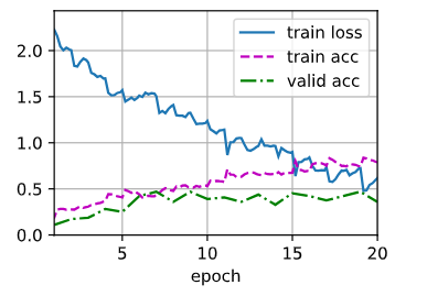
python
# 对测试集进行分类并提交结果
net, preds = get_net(), []
train(net, train_valid_iter, None, num_epochs, lr, wd, devices, lr_period, lr_decay)
for X, _ in test_iter:
    y_hat = net(X.to(devices[0]))
    preds.extend(y_hat.argmax(dim=1).type(torch.int32).cpu().numpy())
sorted_ids = list(range(1,len(test_ds)+1))
sorted_ids.sort(key=lambda x: str(x))
df = pd.DataFrame({'id':sorted_ids,'label':preds})
df['label'] = df['label'].apply(lambda x: train_valid_ds.classes[x])
df.to_csv('submission.csv',index=False)train loss 0.560,train acc 0.805
859.2 examples/sec on [device(type='cuda', index=0)]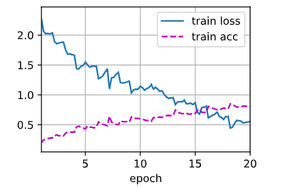
4. 实战Kaggle比赛狗的品种识别ImageNetDogs
整体项目目标:120 类狗狗图像分类比赛 ,用 ** 迁移学习(预训练 ResNet 冻结微调)** 训练,最终生成 Kaggle 可提交的预测 csv 文件;
demo=True用小数据集快速调试,正式跑关闭 demo 用完整数据集。
① 比赛网址是 Checking your browser - reCAPTCHA
python
import os
import torch
import torchvision
from torch import nn
from d2l import torch as d2l
配置小数据集下载(demo 调试模式
d2l.DATA_HUB:注册数据集地址 + MD5 校验码,防止下载文件损坏demo=True:开启小样例数据集(数据量小、训练快,适合学习调试download_extract:自动下载 zip、自动解压,返回解压后的文件夹路径data_dirdemo=False:使用你本地提前下载好的 Kaggle 完整比赛数据集
python
d2l.DATA_HUB['dog_tiny'] = (d2l.DATA_URL + 'kaggle_dog_tiny.zip',
                           '0cb91d09b814ecdc07b50f31f8dcad3e816a86d')

demo = True
if demo:
    data_dir = d2l.download_extract('dog_tiny')
else:
data_dir = os.path_join('..','data','dog_breed-identification')Downloading ..\data\kaggle_dog_tiny.zip from http://d2l-data.s3-accelerate.amazonaws.com/kaggle_dog_tiny.zip...数据集整理函数 reorg_dog_data
1. 函数形参:
data_dir
含义:数据集根目录路径(文件夹地址字符串)
来源:前面代码
data_dir = d2l.download_extract('dog_tiny')得到举例:
'C:/xxx/data/kaggle_dog_tiny'这个文件夹内部一开始有:
labels.csv、train文件夹(所有训练图片)、test文件夹(所有测试图片)2. 函数形参:
valid_ratio
- 英文直译:validation ratio,验证集比例
- 作用:把原始训练图片拆分两部分:训练集 + 验证集
- 比如
valid_ratio=0.1= 拿全部训练图片的 10% 做验证集,剩下 90% 做训练集3. 函数内部变量:
labels
类型:Python 字典
{key: value}key:图片文件名(不带后缀
.jpg)value:该图片对应的狗狗品种名字
来源:从
labels.csv表格读取而来示例内容:
{
    '000bec180eb03b78b2436a80fead340f': 'boston_bull',
    '001513dfcb2ffafc82712f7dcca1c318d': 'dingo',
    ...
}
4. 全局变量:
batch_size
含义:批次大小
深度学习不能一次性把几万张图片全部塞进显卡,会显存爆炸;一次拿
batch_size张图片算一次梯度、更新一次参数三目表达式解释:
batch_size = 32 if demo else 128
demo=True(小数据集调试):batch_size = 32,一次读 32 张图片demo=False(完整大数据集):batch_size = 128,一次读 128 张图片5. 全局变量:
valid_ratio = 0.1给上面函数要用到的验证集比例赋值:划分 10% 数据为验证集
二、逐行拆解函数内部每一行
def reorg_dog_data(data_dir, valid_ratio):
def代表定义自定义函数,函数名叫reorg_dog_data- 函数接收两个输入参数:
- 参数 1:
data_dir数据集根路径- 参数 2:
valid_ratio验证集划分比例- 这个函数整体功能:一键重构、整理整个数据集文件夹结构
第 1 行函数内代码
labels = d2l.read_csv_labels(os.path.join(data_dir,'labels.csv'))①
os.path.join(a, b)路径拼接函数,自动拼接文件夹 + 文件名,避免手动写斜杠
/反斜杠\出错 示例:os.path.join('C:/dogdata', 'labels.csv')→ 拼接出完整路径C:/dogdata/labels.csv②
d2l.read_csv_labels(文件路径)
d2l是李沐动手学深度学习工具库自带函数,专门适配这个狗狗比赛的 csv 文件:
- 打开
labels.csv文件- csv 内部两列:
id(图片名)、breed(品种)- 自动解析成字典,赋值给变量
labels第 2 行函数内代码
d2l.reorg_train_valid(data_dir,labels,valid_ratio)调用 d2l 库内置函数,拆分 + 整理带标签的训练图片,详细过程:
- 读取原始
train文件夹里所有图片- 借助
labels字典知道每张图片是什么品种- 按照
valid_ratio比例随机拆分:
- 90% 图片 → 放到
train_valid_test/train/对应品种文件夹(训练集)- 10% 图片 → 放到
train_valid_test/valid/对应品种文件夹(验证集)- 全部原始训练图合并一份 →
train_valid_test/train_valid/对应品种文件夹(全集,后期用来最终训练)
python
# 整理数据集
def reorg_dog_data(data_dir, valid_ratio):
    labels = d2l.read_csv_labels(os.path.join(data_dir,'labels.csv'))
    d2l.reorg_train_valid(data_dir,labels,valid_ratio)
    d2l.reorg_test(data_dir)

batch_size = 32 if demo else 128
valid_ratio = 0.1
reorg_dog_data(data_dir, valid_ratio)
图像预处理 + 图像增广 ,分为训练集变换 transform_train、测试集变换 transform_test
- transform 是什么 图片不能直接丢进神经网络,必须统一尺寸、转成张量、归一化;
transform就是图片预处理流水线。- 为什么要分 train 和 test 两套 transform?
- 训练集:要做随机增广(随机裁剪、翻转、调色),增加数据多样性,防止过拟合
- 测试集:不能带任何随机操作,保证每次预测结果稳定
逐行拆解 transform_train(训练集预处理)
1. 外层容器 Compose
transform_train = torchvision.transforms.Compose([操作1,操作2,操作3...])
- 变量名:
transform_train,专门给训练集图片使用的预处理规则Compose([]):把括号里面多个图像处理步骤按顺序串行执行,打包成一个整体变换对象操作 1:RandomResizedCrop 随机缩放裁剪
python
运行
torchvision.transforms.RandomResizedCrop(224,scale=(0.08,1.0),ratio=(3.0/4.0, 4.0/3.0))逐个参数拆解:
224:最终裁剪输出图片尺寸 224×224(ResNet 模型固定输入尺寸)scale=(0.08, 1.0): 先在原图上随机截取一块区域,这块区域面积是原图面积的 8% ~ 100% 截取小区域迫使模型学习局部特征,提升泛化能力ratio=(3/4, 4/3): 随机截取区域宽高比在 0.75 ~ 1.33 之间,避免裁剪出极端细长图片- 整体流程:随机裁一块区域 → 拉伸缩放到 224×224
操作 2:RandomHorizontalFlip 随机水平翻转
python
运行
torchvision.transforms.RandomHorizontalFlip()
- 默认概率 0.5:每张图片有 50% 概率左右镜像翻转
- 狗朝左、朝右都是同一个品种,扩充样本多样性,最简单有效的数据增广
操作 3:ColorJitter 随机色彩抖动
python
运行
torchvision.transforms.ColorJitter(brightness=0.4,contrast=0.4,saturation=0.4)随机轻微修改图片属性,模拟拍照光线不同场景:
brightness=0.4:亮度随机浮动 ±40%contrast=0.4:对比度随机浮动 ±40%saturation=0.4:饱和度随机浮动 ±40% 不修改色相(色调),避免改变狗狗本身颜色特征。操作 4:ToTensor () 转张量
python
运行
torchvision.transforms.ToTensor()
- 原始图片是 PIL 图片,像素范围
[0, 255]整数- 转为 PyTorch 张量 Tensor,维度
(通道C, 高度H, 宽度W)- 像素值自动除以 255,归一到
[0, 1]浮点数维度变化举例:(H,W,C) → (C,H,W),符合卷积网络输入格式要求
操作 5:Normalize 标准化(最重要)
python
运行
torchvision.transforms.Normalize([0.485,0.456,0.406], [0.229,0.224,0.225])公式: \(x_{out}=\frac{x-\mu}{\sigma}\)
- 第一个列表
[0.485,0.456,0.406]:RGB 三通道均值 mean- 第二个列表
[0.229,0.224,0.225]:RGB 三通道标准差 std为什么固定这组数值?
这是 ImageNet 数据集全局统计均值方差,我们要用预训练 ResNet,预训练时人家就是用这个归一化; 前后归一化规则必须一模一样,否则模型提取特征完全错乱,准确率暴跌。
python
# 图像增广
transform_train = torchvision.transforms.Compose([
    torchvision.transforms.RandomResizedCrop(224,scale=(0.08,1.0),ratio=(3.0/4.0, 4.0/3.0)),
    torchvision.transforms.RandomHorizontalFlip(),
    torchvision.transforms.ColorJitter(brightness=0.4,contrast=0.4,saturation=0.4),
    torchvision.transforms.ToTensor(),
    torchvision.transforms.Normalize([0.485,0.456,0.406],
                                    [0.229,0.224,0.225])])

transform_test = torchvision.transforms.Compose([
    torchvision.transforms.Resize(256),
    torchvision.transforms.CenterCrop(224),
    torchvision.transforms.ToTensor(),
    torchvision.transforms.Normalize([0.485,0.456,0.406],
                                     [0.229,0.224,0.225])])
变量名 类型 用途 使用哪个 transform train_ds Dataset 数据集对象 划分后的训练集 transform_train(带增广) train_valid_ds Dataset 数据集对象 训练 + 验证全集 transform_train valid_ds Dataset 数据集对象 验证集(看过拟合) transform_test(无增广) test_ds Dataset 数据集对象 比赛测试集,用来预测 transform_test train_iter DataLoader 迭代器 分批读取 train_ds - train_valid_iter DataLoader 迭代器 分批读取全集 - valid_iter DataLoader 迭代器 分批读取验证集 - test_iter DataLoader 迭代器 分批读取测试集 -
创建数据集 Dataset + 数据加载器 DataLoader
python
train_ds, train_valid_ds = [
    torchvision.datasets.ImageFolder(
        os.path.join(data_dir,'train_valid_test',folder),
        transform=transform_train) for folder in ['train','train_valid']]

valid_ds, test_ds = [
    torchvision.datasets.ImageFolder(
    os.path.join(data_dir,'train_valid_test',folder),
    transform=transform_test) for folder in ['valid','test']]

train_iter, train_valid_iter = [
    torch.utils.data.DataLoader(dataset,batch_size,shuffle=True,drop_last=True) for dataset in (train_ds, train_valid_ds)]

valid_iter = torch.utils.data.DataLoader(valid_ds,batch_size,shuffle=False,drop_last=True)
test_iter = torch.utils.data.DataLoader(test_ds,batch_size,shuffle=False,drop_last=False)
python
# 微调预训练模型
# 除了最后一层外,前面的层固定住参数不变
def get_net(device):
    finetune_net = nn.Sequential()
    finetune_net.features = torchvision.models.resnet34(pretrained=True)
    print("finetune_net:", finetune_net)
    finetune_net.output_new = nn.Sequential(nn.Linear(1000,256),nn.ReLU(),nn.Linear(256,120)) #  在原始网络后又加了一层
    print("finetune_net:", finetune_net)
    finetune_net = finetune_net.to(devices[0])
    for param in finetune_net.features.parameters(): # 遍历features的所有参数
        param.requires_grad = False
    return finetune_net # 返回整个网络,这个网络中原始层的参数固定住了,保持不变
python
# 计算损失
loss = nn.CrossEntropyLoss(reduction='none')

def evaluate_loss(data_iter, net, devices):
    l_sum, n = 0.0, 0
    for features, labels in data_iter:
        features, labels = features.to(devices[0]), labels.to(devices[0])
        outputs = net(features)
        l = loss(outputs, labels)
        l_sum += l.sum()
        n += labels.numel()
    return l_sum / n
python
# 训练函数
def train(net, train_iter, valid_iter, num_epochs, lr, wd, devices, lr_period,lr_decay):
    net = nn.DataParallel(net,device_ids=devices).to(devices[0])
    trainer = torch.optim.SGD(
        (param for param in net.parameters() if param.requires_grad),
        lr = lr, momentum = 0.9, weight_decay=wd)
    scheduler = torch.optim.lr_scheduler.StepLR(trainer, lr_period, lr_decay)
    num_batches, timer = len(train_iter), d2l.Timer()
    legend = ['train loss']
    if valid_iter is not None:
        legend.append('valid loss')
    animator = d2l.Animator(xlabel='epoch',xlim=[1,num_epochs],legend=legend)

    for epoch in range(num_epochs):
        metric = d2l.Accumulator(2)
        for i, (features, labels) in enumerate(train_iter):
            timer.start()
            features, labels = features.to(devices[0]), labels.to(devices[0])
            trainer.zero_grad()
            output = net(features)
            l = loss(output, labels).sum()
            l.backward()
            trainer.step()
            metric.add(l,labels.shape[0])
            timer.stop()
            if (i+1) % (num_batches // 5) == 0 or i == num_batches -1:
                animator.add(epoch + (i+1) / num_batches,
                             (metric[0] / metric[1], None))
        measures = f'train loss {metric[0] / metric[1]:.3f}'
        if valid_iter is not None:
            valid_loss = evaluate_loss(valid_iter, net, devices)
            animator.add(epoch + 1, (None, valid_loss.detach()))
        scheduler.step()
    if valid_iter is not None:
        measures += f', valid loss {valid_loss:.3f}'
    print(measures + f'\n{metric[1] * num_epochs / timer.sum():.1f}'
         f' examples/sec on {str(devices)}')
python
devices, num_epochs, lr, wd = d2l.try_all_gpus(), 10, 1e-4, 1e-4
lr_period, lr_decay, net = 2, 0.9, get_net(devices)
train(net, train_iter, valid_iter, num_epochs, lr, wd, devices, lr_period, lr_decay) train loss 1.119, valid loss 1.561
569.0 examples/sec on [device(type='cuda', index=0)]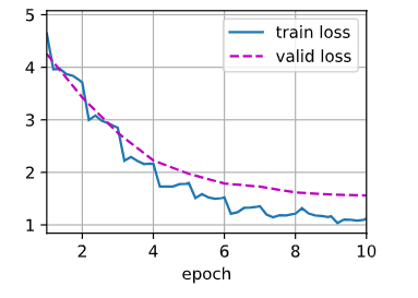
python
net = get_net(devices)
train(net, train_valid_iter, None, num_epochs, lr, wd, devices, lr_period, lr_decay) train loss 1.068
761.3 examples/sec on [device(type='cuda', index=0)]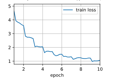
python
preds = []
for data, label in test_iter:
    # 计算每一个样本对每一类的概率是多少
    output = torch.nn.functional.softmax(net(data.to(devices[0])), dim=0)
    preds.extend(output.cpu().detach().numpy())
    print(len(preds))
ids = sorted(os.listdir(os.path.join(data_dir, 'train_valid_test', 'test', 'unknown')))
with open('submission.csv','w') as f:
    f.write('id,' + ','.join(train_valid_ds.classes)+'\n')
    for i, output in zip(ids, preds):
f.write(i.split('.')[0] + ',' + ','.join([str(num) for num in output]) + '\n') 105. 目标检测
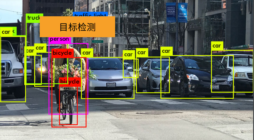
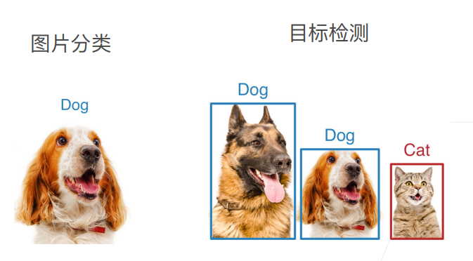
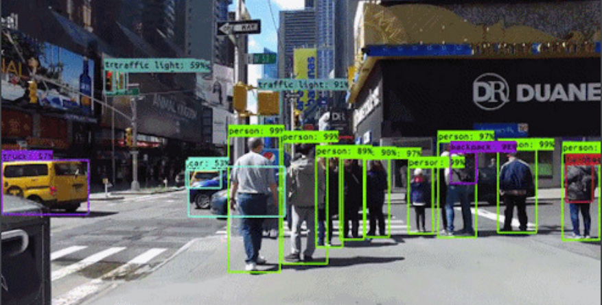
1. 总结

2. 目标检测和边界框
python
%matplotlib inline
import torch
from d2l import torch as d2l

d2l.set_figsize()
img = d2l.plt.imread('01_Data/img/catdog.jpg')
d2l.plt.imshow(img)<matplotlib.image.AxesImage at 0x19a816c4a90>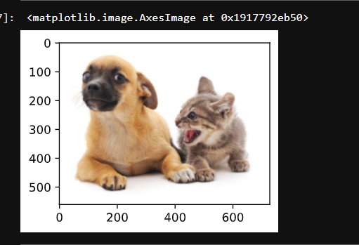
python
# 定义在这两种表示之间进行转换的函数
def box_corner_to_center(boxes):
    """从(左上,右下)转换到(中间,宽度,高度)"""
    x1, y1, x2, y2 = boxes[:,0], boxes[:,1], boxes[:,2], boxes[:,3]
    cx = (x1 + x2) / 2
    cy = (y1 + y2) / 2
    w  = x2 - x1
    h  = y2 - y1
    boxes = torch.stack((cx,cy,w,h),axis = -1)
    return boxes

def box_center_to_corner(boxes):
    """从(中间,宽度,高度)转换到(左上,右下)"""
    cx, cy, w, h = boxes[:,0], boxes[:,1], boxes[:,2], boxes[:,3]
    x1 = cx - 0.5 * w
    y1 = cy - 0.5 * h
    x2 = cx + 0.5 * w
    y2 = cy + 0.5 * h
    boxes = torch.stack((x1,y1,x2,y2),axis = -1)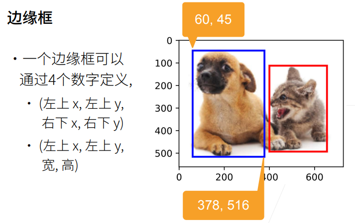
return boxes构造猫狗两个边界框,测试坐标互转函数是否写对,来回转换后和原框一致,代表转换逻辑没问题。
python
# 定义图像中狗和猫的边界框
dog_bbox, cat_bbox = [60.0, 45.0, 378.0, 516.0], [400.0, 112.0, 655.0, 493.0]
#把两个框打包成嵌套列表,并把普通 Python 列表,转成 PyTorch 张量(神经网络专用数组)
boxes = torch.tensor((dog_bbox,cat_bbox))
# boxes 转中间表示,再转回来,等于自己
box_center_to_corner(box_corner_to_center(boxes)) == boxes tensor([[True, True, True, True],
[True, True, True, True]])目标:在图片上画两个方框,蓝框圈狗、红框圈猫
fill=False fill = 填充;False = 矩形内部不填充颜色,只画空心边框 如果写 True,整个框内部会被颜色糊住,挡住图片里的猫狗。
fig.axesaxes = 坐标轴区域,一张图的绘图区域,所有线条、方框都要添加到 axes 上才看得见。- patch matplotlib 里,线条、矩形、圆形这类几何图形都叫 patch(图形补丁),
add_patch就是往图上加几何图形。
python
# 将边界框在图中画出
def bbox_to_rect(bbox,color):
    return d2l.plt.Rectangle(xy=(bbox[0],bbox[1]),width=bbox[2]-bbox[0],
                            height=bbox[3] - bbox[1], fill=False,
                            edgecolor=color,linewidth=2)

fig = d2l.plt.imshow(img)
fig.axes.add_patch(bbox_to_rect(dog_bbox,'blue'))
fig.axes.add_patch(bbox_to_rect(cat_bbox,'red'))<matplotlib.patches.Rectangle at 0x19a8178f9b0>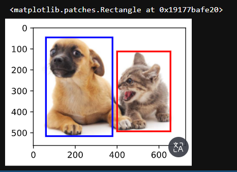
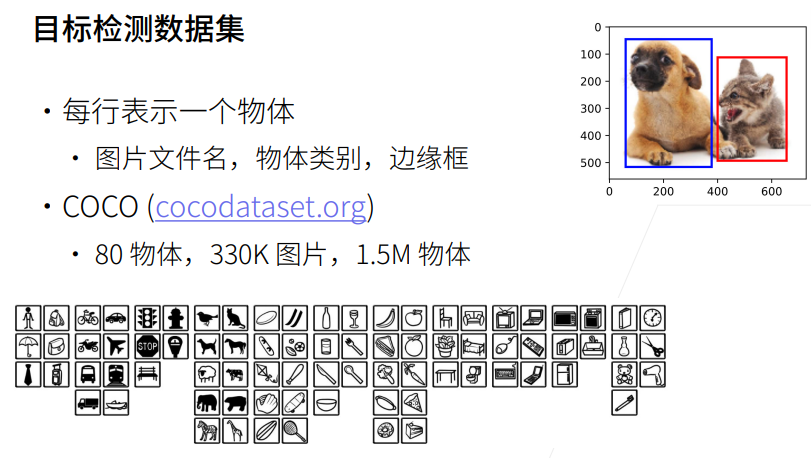
3. 目标检测数据集
整体作用:注册香蕉目标检测数据集的下载地址 + 校验码,为后续自动下载数据集做准备
1、先搞懂
d2l.DATA_HUB是什么
DATA_HUB是 d2l 库内置的字典 格式:数据集名字 : (下载网址, MD5校验码)作用:给数据集起别名,后面调用d2l.download_extract('banana-detection')时,程序自动去这个地址下载压缩包2、拆分括号里两个元素
① 第一个元素:下载地址
plaintext
d2l.DATA_URL + 'banana-detection.zip'
d2l.DATA_URL是 d2l 预设好的云端根地址- 拼接后 = 香蕉数据集压缩包完整网络下载链接
② 第二个长字符串:MD5 校验码
'5de25c8fce5ccdea9f91267273465dc968d20d72'
- 作用:校验下载文件完整性
- 如果下载中途断网、文件损坏,MD5 比对不一致,d2l 会提示文件异常,避免用破损数据集训练报错
3、整行赋值含义
往
DATA_HUB字典里新增一条记录:
- 数据集别名:
banana-detection- 对应资源:香蕉检测数据集压缩包 + 校验码
python
%matplotlib inline
import os
import pandas as pd
import torch
import torchvision
from d2l import torch as d2l

d2l.DATA_HUB['banana-detection'] = (d2l.DATA_URL + 'banana-detection.zip','5de25c8fce5ccdea9f91267273465dc968d20d72')自动下载香蕉数据集,读取所有图片 + 每张图里香蕉的边界框标签,最后做格式整理、坐标归一化,返回给后面训练用。
download_extract 作用:
- 先检查本地有没有下载解压好的数据集
- 没有就自动下载 zip 包、自动解压
- 返回解压后的总文件夹路径 ,存到变量
data_dir**os.join(a,b,c):**自动拼接路径,避免斜杠正反写错
- .iterrows():pandas 遍历表格每一行的方法
- 每次循环得到两个变量:
img_name:当前行索引 = 图片名字(比如0.png、1.png)target:当前行剩下全部内容(类别 + x1,y1,x2,y2 五个数字)返回两个东西:
images:列表,每个元素是单张图片张量- 处理好的标签张量,形状
[N, 1, 5],坐标归一化到 0~1整段函数完整流程总结
- 根据
is_train判断读训练集还是验证集- 自动下载 / 定位数据集,找到标签 label.csv
- 读取表格,图片名和标签一一绑定
- 循环:读每张图片存列表、读对应标签存列表
- 打印一堆信息调试查看数据结构
- 标签转张量、增加维度适配检测网络、坐标除以 256 归一化
- 返回图片列表 + 规整好的标签张量
补充小疑问:为什么要 unsqueeze (1) 多一维?
如果形状
[N,5],只能代表 "每张图 5 个数字"; 改成[N,1,5]语义清晰:每张图有 1 个物体框,每个框 5 个参数 ,以后拓展到一张图多个物体(比如 3 根香蕉,写成[N,3,5])代码不用大改,是目标检测通用格式。
python
# 读取香蕉检测数据集
def read_data_bananas(is_train=True):
    """读取香蕉检测数据集中的图像和标签"""
#download_extract先检查本地有没有下载解压好的数据集,没有再自动下载
    data_dir = d2l.download_extract('banana-detection')
#csv_fname 就是标签文件 label.csv 的完整路径
    csv_fname = os.path.join(data_dir,
                            'bananas_train' if is_train else 'bananas_val',
                            'label.csv')
    csv_data = pd.read_csv(csv_fname)
    csv_data = csv_data.set_index('img_name')
    images, targets = [], []#创建两个空列表,存图片、存标签
    # 把图片、标号全部读到内存里面
    for img_name, target in csv_data.iterrows():#按行遍历
        #.append(...):把读好的图片放进 images 列表
        images.append(torchvision.io.read_image(os.path.join(data_dir,'bananas_train' if is_train else 'bananas_val','images',f'{img_name}')))
        targets.append(list(target))
    print("len(targets):",len(targets))#打印一共有多少张图片(多少组标签)
    print("len(targets[0]):",len(targets[0]))#打印第一张图片标签长度:固定是 5:[类别, x1, y1, x2, y2]
    #打印第一张标签五个数字分别是什么,直观看到类别、四个坐标
    print("targets[0][0]....targets[0][4]:",targets[0][0], targets[0][1], targets[0][2], targets[0][3], targets[0][4])
    print("type(targets):",type(targets))
#把嵌套列表转张量;.unsqueeze(1):在第1维新增一个长度为 1 的维度
print("torch.tensor(targets).unsqueeze(1).shape:",torch.tensor(targets).unsqueeze(1).shape) # unsqueeze函数在指定位置加上维数为一的维度
#坐标归一化
    print("len(torch.tensor(targets).unsqueeze(1) / 256):", len(torch.tensor(targets).unsqueeze(1) / 256))
    print("type(torch.tensor(targets).unsqueeze(1) / 256):", type(torch.tensor(targets).unsqueeze(1) / 256))
    return images, torch.tensor(targets).unsqueeze(1) / 256 # 归一化使得收敛更快
python
# 创建一个自定义Dataset实例
class BananasDataset(torch.utils.data.Dataset):
    """一个用于加载香蕉检测数据集的自定义数据集"""
    def __init__(self, is_train):
        self.features, self.labels = read_data_bananas(is_train)
        print('read ' + str(len(self.features)) + (f' training examples' if is_train else f'validation examples'))

    def __getitem__(self, idx):
        return (self.features[idx].float(), self.labels[idx])

    def __len__(self):
        return len(self.features)
python
# 为训练集和测试集返回两个数据加载器实例
def load_data_bananas(batch_size):
    """加载香蕉检测数据集"""
    train_iter = torch.utils.data.DataLoader(BananasDataset(is_train=True),
                                            batch_size, shuffle=True)
    val_iter = torch.utils.data.DataLoader(BananasDataset(is_train=False),
                                          batch_size)
    return train_iter, val_iter
python
# 读取一个小批量,并打印其中的图像和标签的形状
batch_size, edge_size = 32, 256
train_iter, _ = load_data_bananas(batch_size)
batch = next(iter(train_iter))
# ([32,1,5]) 中的1是每张图片中有几种类别,这里只有一种香蕉要识别的类别
# 5是类别标号、框的四个参数
batch[0].shape, batch[1].shapeDownloading ..\data\banana-detection.zip from http://d2l-data.s3-accelerate.amazonaws.com/banana-detection.zip...
len(targets): 1000
len(targets[0]): 5
targets[0][0]....targets[0][4]: 0 104 20 143 58
type(targets): <class 'list'>
torch.tensor(targets).unsqueeze(1).shape: torch.Size([1000, 1, 5])
len(torch.tensor(targets).unsqueeze(1) / 256): 1000
type(torch.tensor(targets).unsqueeze(1) / 256): <class 'torch.Tensor'>
read 1000 training examples
Downloading ..\data\banana-detection.zip from http://d2l-data.s3-accelerate.amazonaws.com/banana-detection.zip...
len(targets): 100
len(targets[0]): 5
targets[0][0]....targets[0][4]: 0 183 63 241 112
type(targets): <class 'list'>
torch.tensor(targets).unsqueeze(1).shape: torch.Size([100, 1, 5])
len(torch.tensor(targets).unsqueeze(1) / 256): 100
type(torch.tensor(targets).unsqueeze(1) / 256): <class 'torch.Tensor'>
read 100validation examples(torch.Size([32, 3, 256, 256]), torch.Size([32, 1, 5]))
python
# 示例
# pytorch里permute是改变参数维度的函数,
# Dataset里读的img维度是[batch_size, RGB, h, w],
# 但是plt画图的时候要求是[h, w, RGB],所以要调整一下

# 做图片的时候,一般是会用一个ToTensor()将图片归一化到【0, 1】,这样收敛更快
print("原始图片:\n", batch[0][0])
print("原始图片:\n", (batch[0][0:10].permute(0,2,3,1)))
print("归一化后图片:\n", (batch[0][0:10].permute(0,2,3,1)) / 255 )
imgs = (batch[0][0:10].permute(0,2,3,1)) / 255
#imgs = (batch[0][0:10].permute(0,2,3,1))
# d2l.show_images输入的imgs图片参数是归一化后的图片
axes = d2l.show_images(imgs, 2, 5, scale=2)
for ax, label in zip(axes, batch[1][0:10]):
d2l.show_bboxes(ax, [label[0][1:5] * edge_size], colors=['w'])原始图片:
tensor([[[248., 249., 250., ..., 193., 194., 193.],
[245., 244., 243., ..., 195., 197., 196.],
[243., 243., 241., ..., 197., 200., 201.],
...,
[ 17., 10., 13., ..., 92., 112., 119.],
[ 19., 14., 12., ..., 114., 115., 113.],
[ 13., 22., 12., ..., 98., 104., 118.]],
[[252., 253., 252., ..., 206., 207., 206.],
[249., 248., 245., ..., 205., 207., 206.],
[245., 245., 243., ..., 206., 209., 210.],
...,
[ 12., 5., 8., ..., 82., 102., 109.],
[ 14., 9., 7., ..., 105., 106., 104.],
[ 8., 17., 7., ..., 91., 95., 109.]],
[[251., 252., 251., ..., 215., 216., 215.],
[248., 247., 244., ..., 214., 216., 215.],
[244., 244., 242., ..., 213., 216., 217.],
...,
[ 6., 0., 2., ..., 72., 92., 99.],
[ 8., 3., 1., ..., 96., 97., 95.],
[ 2., 11., 1., ..., 81., 86., 100.]]])
原始图片:
tensor([[[[248., 252., 251.],
[249., 253., 252.],
[250., 252., 251.],
...,
[193., 206., 215.],
[194., 207., 216.],
[193., 206., 215.]],
[[245., 249., 248.],
[244., 248., 247.],
[243., 245., 244.],
...,
[195., 205., 214.],
[197., 207., 216.],
[196., 206., 215.]],
[[243., 245., 244.],
[243., 245., 244.],
[241., 243., 242.],
...,
[197., 206., 213.],
[200., 209., 216.],
[201., 210., 217.]],
...,
[[ 17., 12., 6.],
[ 10., 5., 0.],
[ 13., 8., 2.],
...,
[ 92., 82., 72.],
[112., 102., 92.],
[119., 109., 99.]],
[[ 19., 14., 8.],
[ 14., 9., 3.],
[ 12., 7., 1.],
...,
[114., 105., 96.],
[115., 106., 97.],
[113., 104., 95.]],
[[ 13., 8., 2.],
[ 22., 17., 11.],
[ 12., 7., 1.],
...,
[ 98., 91., 81.],
[104., 95., 86.],
[118., 109., 100.]]],
[[[180., 167., 132.],
[177., 163., 128.],
[169., 153., 117.],
...,
[172., 140., 102.],
[168., 138., 100.],
[165., 135., 97.]],
[[186., 173., 138.],
[181., 167., 130.],
[176., 158., 122.],
...,
[171., 139., 101.],
[170., 138., 100.],
[166., 136., 98.]],
[[187., 173., 136.],
[181., 167., 128.],
[175., 157., 119.],
...,
[172., 139., 104.],
[172., 139., 104.],
[170., 137., 102.]],
...,
[[173., 148., 118.],
[146., 121., 91.],
[173., 148., 117.],
...,
[182., 151., 131.],
[138., 106., 83.],
[142., 110., 85.]],
[[ 80., 60., 33.],
[151., 132., 102.],
[193., 174., 142.],
...,
[215., 194., 175.],
[117., 95., 71.],
[139., 118., 91.]],
[[129., 113., 87.],
[110., 95., 66.],
[119., 102., 72.],
...,
[141., 124., 104.],
[164., 146., 122.],
[181., 164., 136.]]],
[[[169., 146., 50.],
[182., 157., 64.],
[187., 160., 69.],
...,
[ 85., 68., 40.],
[145., 133., 107.],
[253., 246., 220.]],
[[162., 139., 45.],
[163., 138., 46.],
[169., 142., 55.],
...,
[127., 107., 80.],
[157., 145., 119.],
[249., 242., 216.]],
[[163., 137., 50.],
[160., 134., 47.],
[177., 149., 66.],
...,
[138., 117., 90.],
[156., 141., 118.],
[254., 243., 221.]],
...,
[[ 18., 19., 11.],
[ 11., 12., 4.],
[ 13., 14., 6.],
...,
[ 49., 48., 17.],
[ 90., 88., 63.],
[248., 246., 225.]],
[[ 13., 16., 5.],
[ 11., 14., 3.],
[ 18., 20., 9.],
...,
[ 38., 39., 8.],
[ 86., 85., 64.],
[245., 244., 226.]],
[[ 11., 15., 1.],
[ 8., 12., 0.],
[ 18., 20., 9.],
...,
[ 35., 38., 9.],
[ 88., 87., 67.],
[249., 247., 232.]]],
...,
[[[158., 108., 35.],
[153., 108., 43.],
[101., 67., 22.],
...,
[129., 125., 87.],
[189., 184., 164.],
[226., 220., 208.]],
[[164., 115., 36.],
[106., 62., 0.],
[107., 70., 18.],
...,
[118., 115., 80.],
[173., 168., 146.],
[151., 148., 131.]],
[[203., 154., 62.],
[184., 137., 55.],
[109., 65., 2.],
...,
[176., 172., 145.],
[195., 195., 169.],
[116., 116., 92.]],
...,
[[ 99., 47., 10.],
[134., 87., 57.],
[ 64., 27., 9.],
...,
[201., 140., 57.],
[146., 87., 7.],
[167., 108., 30.]],
[[ 71., 28., 0.],
[137., 99., 50.],
[ 83., 53., 17.],
...,
[214., 153., 70.],
[182., 122., 34.],
[168., 109., 17.]],
[[ 89., 51., 0.],
[170., 135., 77.],
[134., 107., 62.],
...,
[195., 134., 51.],
[182., 123., 31.],
[209., 151., 52.]]],
[[[196., 198., 97.],
[178., 180., 79.],
[194., 194., 98.],
...,
[116., 74., 34.],
[ 76., 42., 4.],
[ 61., 33., 0.]],
[[198., 201., 98.],
[190., 193., 90.],
[191., 193., 92.],
...,
[108., 67., 23.],
[101., 68., 23.],
[103., 75., 28.]],
[[206., 209., 104.],
[195., 198., 91.],
[181., 185., 75.],
...,
[123., 84., 29.],
[171., 136., 80.],
[177., 144., 90.]],
...,
[[131., 127., 64.],
[130., 129., 65.],
[125., 126., 60.],
...,
[ 93., 112., 20.],
[ 93., 110., 16.],
[101., 118., 24.]],
[[130., 124., 64.],
[132., 128., 65.],
[126., 126., 62.],
...,
[ 96., 115., 23.],
[100., 119., 27.],
[104., 123., 31.]],
[[126., 120., 60.],
[129., 125., 64.],
[127., 126., 62.],
...,
[108., 127., 35.],
[112., 131., 39.],
[110., 129., 37.]]],
[[[ 57., 82., 40.],
[ 62., 87., 45.],
[ 39., 65., 26.],
...,
[244., 253., 232.],
[ 94., 108., 83.],
[133., 149., 122.]],
[[ 55., 80., 38.],
[ 63., 88., 46.],
[ 33., 60., 19.],
...,
[207., 216., 199.],
[118., 132., 109.],
[ 57., 73., 46.]],
[[ 41., 66., 24.],
[ 39., 64., 22.],
[ 41., 66., 24.],
...,
[235., 241., 231.],
[ 86., 99., 79.],
[ 48., 66., 40.]],
...,
[[ 68., 90., 44.],
[ 63., 85., 38.],
[ 53., 73., 22.],
...,
[ 56., 71., 42.],
[ 52., 65., 39.],
[ 37., 50., 24.]],
[[ 46., 67., 24.],
[ 63., 82., 37.],
[ 50., 67., 22.],
...,
[ 45., 59., 33.],
[ 52., 64., 40.],
[ 35., 47., 23.]],
[[ 44., 65., 24.],
[ 44., 62., 20.],
[ 55., 72., 28.],
...,
[ 49., 63., 37.],
[ 40., 52., 30.],
[ 39., 51., 29.]]]])
归一化后图片:
tensor([[[[0.9725, 0.9882, 0.9843],
[0.9765, 0.9922, 0.9882],
[0.9804, 0.9882, 0.9843],
...,
[0.7569, 0.8078, 0.8431],
[0.7608, 0.8118, 0.8471],
[0.7569, 0.8078, 0.8431]],
[[0.9608, 0.9765, 0.9725],
[0.9569, 0.9725, 0.9686],
[0.9529, 0.9608, 0.9569],
...,
[0.7647, 0.8039, 0.8392],
[0.7725, 0.8118, 0.8471],
[0.7686, 0.8078, 0.8431]],
[[0.9529, 0.9608, 0.9569],
[0.9529, 0.9608, 0.9569],
[0.9451, 0.9529, 0.9490],
...,
[0.7725, 0.8078, 0.8353],
[0.7843, 0.8196, 0.8471],
[0.7882, 0.8235, 0.8510]],
...,
[[0.0667, 0.0471, 0.0235],
[0.0392, 0.0196, 0.0000],
[0.0510, 0.0314, 0.0078],
...,
[0.3608, 0.3216, 0.2824],
[0.4392, 0.4000, 0.3608],
[0.4667, 0.4275, 0.3882]],
[[0.0745, 0.0549, 0.0314],
[0.0549, 0.0353, 0.0118],
[0.0471, 0.0275, 0.0039],
...,
[0.4471, 0.4118, 0.3765],
[0.4510, 0.4157, 0.3804],
[0.4431, 0.4078, 0.3725]],
[[0.0510, 0.0314, 0.0078],
[0.0863, 0.0667, 0.0431],
[0.0471, 0.0275, 0.0039],
...,
[0.3843, 0.3569, 0.3176],
[0.4078, 0.3725, 0.3373],
[0.4627, 0.4275, 0.3922]]],
[[[0.7059, 0.6549, 0.5176],
[0.6941, 0.6392, 0.5020],
[0.6627, 0.6000, 0.4588],
...,
[0.6745, 0.5490, 0.4000],
[0.6588, 0.5412, 0.3922],
[0.6471, 0.5294, 0.3804]],
[[0.7294, 0.6784, 0.5412],
[0.7098, 0.6549, 0.5098],
[0.6902, 0.6196, 0.4784],
...,
[0.6706, 0.5451, 0.3961],
[0.6667, 0.5412, 0.3922],
[0.6510, 0.5333, 0.3843]],
[[0.7333, 0.6784, 0.5333],
[0.7098, 0.6549, 0.5020],
[0.6863, 0.6157, 0.4667],
...,
[0.6745, 0.5451, 0.4078],
[0.6745, 0.5451, 0.4078],
[0.6667, 0.5373, 0.4000]],
...,
[[0.6784, 0.5804, 0.4627],
[0.5725, 0.4745, 0.3569],
[0.6784, 0.5804, 0.4588],
...,
[0.7137, 0.5922, 0.5137],
[0.5412, 0.4157, 0.3255],
[0.5569, 0.4314, 0.3333]],
[[0.3137, 0.2353, 0.1294],
[0.5922, 0.5176, 0.4000],
[0.7569, 0.6824, 0.5569],
...,
[0.8431, 0.7608, 0.6863],
[0.4588, 0.3725, 0.2784],
[0.5451, 0.4627, 0.3569]],
[[0.5059, 0.4431, 0.3412],
[0.4314, 0.3725, 0.2588],
[0.4667, 0.4000, 0.2824],
...,
[0.5529, 0.4863, 0.4078],
[0.6431, 0.5725, 0.4784],
[0.7098, 0.6431, 0.5333]]],
[[[0.6627, 0.5725, 0.1961],
[0.7137, 0.6157, 0.2510],
[0.7333, 0.6275, 0.2706],
...,
[0.3333, 0.2667, 0.1569],
[0.5686, 0.5216, 0.4196],
[0.9922, 0.9647, 0.8627]],
[[0.6353, 0.5451, 0.1765],
[0.6392, 0.5412, 0.1804],
[0.6627, 0.5569, 0.2157],
...,
[0.4980, 0.4196, 0.3137],
[0.6157, 0.5686, 0.4667],
[0.9765, 0.9490, 0.8471]],
[[0.6392, 0.5373, 0.1961],
[0.6275, 0.5255, 0.1843],
[0.6941, 0.5843, 0.2588],
...,
[0.5412, 0.4588, 0.3529],
[0.6118, 0.5529, 0.4627],
[0.9961, 0.9529, 0.8667]],
...,
[[0.0706, 0.0745, 0.0431],
[0.0431, 0.0471, 0.0157],
[0.0510, 0.0549, 0.0235],
...,
[0.1922, 0.1882, 0.0667],
[0.3529, 0.3451, 0.2471],
[0.9725, 0.9647, 0.8824]],
[[0.0510, 0.0627, 0.0196],
[0.0431, 0.0549, 0.0118],
[0.0706, 0.0784, 0.0353],
...,
[0.1490, 0.1529, 0.0314],
[0.3373, 0.3333, 0.2510],
[0.9608, 0.9569, 0.8863]],
[[0.0431, 0.0588, 0.0039],
[0.0314, 0.0471, 0.0000],
[0.0706, 0.0784, 0.0353],
...,
[0.1373, 0.1490, 0.0353],
[0.3451, 0.3412, 0.2627],
[0.9765, 0.9686, 0.9098]]],
...,
[[[0.6196, 0.4235, 0.1373],
[0.6000, 0.4235, 0.1686],
[0.3961, 0.2627, 0.0863],
...,
[0.5059, 0.4902, 0.3412],
[0.7412, 0.7216, 0.6431],
[0.8863, 0.8627, 0.8157]],
[[0.6431, 0.4510, 0.1412],
[0.4157, 0.2431, 0.0000],
[0.4196, 0.2745, 0.0706],
...,
[0.4627, 0.4510, 0.3137],
[0.6784, 0.6588, 0.5725],
[0.5922, 0.5804, 0.5137]],
[[0.7961, 0.6039, 0.2431],
[0.7216, 0.5373, 0.2157],
[0.4275, 0.2549, 0.0078],
...,
[0.6902, 0.6745, 0.5686],
[0.7647, 0.7647, 0.6627],
[0.4549, 0.4549, 0.3608]],
...,
[[0.3882, 0.1843, 0.0392],
[0.5255, 0.3412, 0.2235],
[0.2510, 0.1059, 0.0353],
...,
[0.7882, 0.5490, 0.2235],
[0.5725, 0.3412, 0.0275],
[0.6549, 0.4235, 0.1176]],
[[0.2784, 0.1098, 0.0000],
[0.5373, 0.3882, 0.1961],
[0.3255, 0.2078, 0.0667],
...,
[0.8392, 0.6000, 0.2745],
[0.7137, 0.4784, 0.1333],
[0.6588, 0.4275, 0.0667]],
[[0.3490, 0.2000, 0.0000],
[0.6667, 0.5294, 0.3020],
[0.5255, 0.4196, 0.2431],
...,
[0.7647, 0.5255, 0.2000],
[0.7137, 0.4824, 0.1216],
[0.8196, 0.5922, 0.2039]]],
[[[0.7686, 0.7765, 0.3804],
[0.6980, 0.7059, 0.3098],
[0.7608, 0.7608, 0.3843],
...,
[0.4549, 0.2902, 0.1333],
[0.2980, 0.1647, 0.0157],
[0.2392, 0.1294, 0.0000]],
[[0.7765, 0.7882, 0.3843],
[0.7451, 0.7569, 0.3529],
[0.7490, 0.7569, 0.3608],
...,
[0.4235, 0.2627, 0.0902],
[0.3961, 0.2667, 0.0902],
[0.4039, 0.2941, 0.1098]],
[[0.8078, 0.8196, 0.4078],
[0.7647, 0.7765, 0.3569],
[0.7098, 0.7255, 0.2941],
...,
[0.4824, 0.3294, 0.1137],
[0.6706, 0.5333, 0.3137],
[0.6941, 0.5647, 0.3529]],
...,
[[0.5137, 0.4980, 0.2510],
[0.5098, 0.5059, 0.2549],
[0.4902, 0.4941, 0.2353],
...,
[0.3647, 0.4392, 0.0784],
[0.3647, 0.4314, 0.0627],
[0.3961, 0.4627, 0.0941]],
[[0.5098, 0.4863, 0.2510],
[0.5176, 0.5020, 0.2549],
[0.4941, 0.4941, 0.2431],
...,
[0.3765, 0.4510, 0.0902],
[0.3922, 0.4667, 0.1059],
[0.4078, 0.4824, 0.1216]],
[[0.4941, 0.4706, 0.2353],
[0.5059, 0.4902, 0.2510],
[0.4980, 0.4941, 0.2431],
...,
[0.4235, 0.4980, 0.1373],
[0.4392, 0.5137, 0.1529],
[0.4314, 0.5059, 0.1451]]],
[[[0.2235, 0.3216, 0.1569],
[0.2431, 0.3412, 0.1765],
[0.1529, 0.2549, 0.1020],
...,
[0.9569, 0.9922, 0.9098],
[0.3686, 0.4235, 0.3255],
[0.5216, 0.5843, 0.4784]],
[[0.2157, 0.3137, 0.1490],
[0.2471, 0.3451, 0.1804],
[0.1294, 0.2353, 0.0745],
...,
[0.8118, 0.8471, 0.7804],
[0.4627, 0.5176, 0.4275],
[0.2235, 0.2863, 0.1804]],
[[0.1608, 0.2588, 0.0941],
[0.1529, 0.2510, 0.0863],
[0.1608, 0.2588, 0.0941],
...,
[0.9216, 0.9451, 0.9059],
[0.3373, 0.3882, 0.3098],
[0.1882, 0.2588, 0.1569]],
...,
[[0.2667, 0.3529, 0.1725],
[0.2471, 0.3333, 0.1490],
[0.2078, 0.2863, 0.0863],
...,
[0.2196, 0.2784, 0.1647],
[0.2039, 0.2549, 0.1529],
[0.1451, 0.1961, 0.0941]],
[[0.1804, 0.2627, 0.0941],
[0.2471, 0.3216, 0.1451],
[0.1961, 0.2627, 0.0863],
...,
[0.1765, 0.2314, 0.1294],
[0.2039, 0.2510, 0.1569],
[0.1373, 0.1843, 0.0902]],
[[0.1725, 0.2549, 0.0941],
[0.1725, 0.2431, 0.0784],
[0.2157, 0.2824, 0.1098],
...,
[0.1922, 0.2471, 0.1451],
[0.1569, 0.2039, 0.1176],
[0.1529, 0.2000, 0.1137]]]])b'\r\n\r\n\r\n
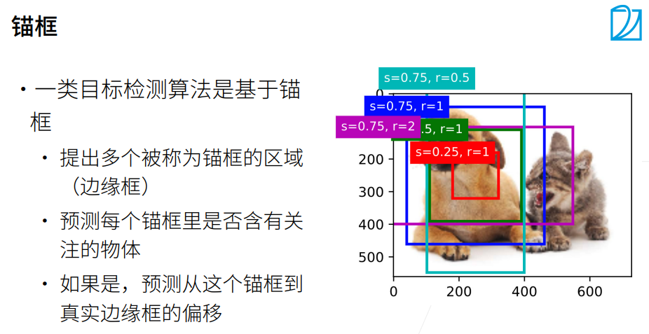
6. 锚框
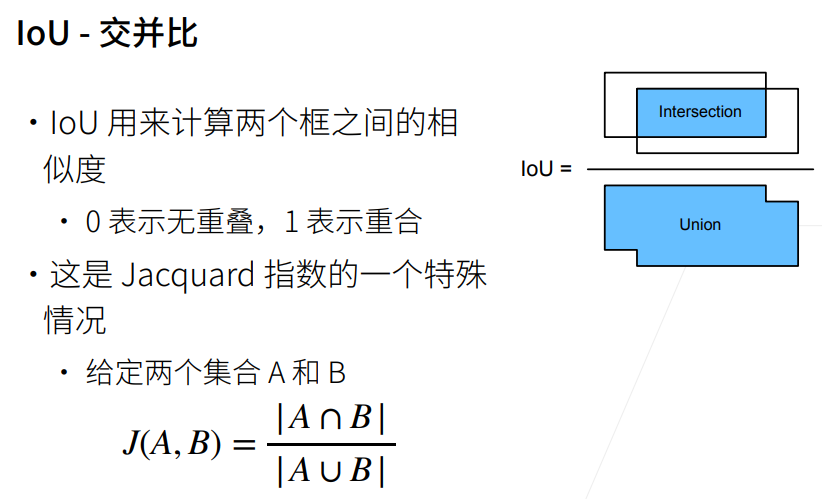
在目标检测任务中,框(即锚框或候选框)的生成是基于预定义的一组尺度和比例进行的,通常是在图像的每个位置生成多个框。这些框的位置和尺度是固定的,但在不同的位置可能有不同的大小和形状。
这些框的生成是为了覆盖不同尺度和形状的目标物体。 然后,生成的每个框都会与真实目标框进行匹配,通过计算它们之间的IoU(交并比)来评估它们的相似度。IoU计算量化了两个框之间的重叠程度,可以判断它们是否匹配。
根据IoU的计算结果,可以进行以下判断和处理:
如果某个框与任何一个真实目标框的IoU超过阈值(通常为0.5或0.7),则认为它与一个真实目标框匹配,被标记为正样本。
如果某个框与所有真实目标框的IoU都小于阈值,则认为它与背景不匹配,被标记为负样本(背景样本)。
如果某个框与某个真实目标框的IoU在阈值范围内,但与其他真实目标框的IoU也很接近,则可以将它忽略,不参与训练和评估。
根据这样的匹配和判断过程,可以确定哪些锚框是与真实目标框匹配的正样本,哪些是与背景不匹配的负样本,以及哪些可以被忽略。
通过这种方式,模型可以学习到目标物体的定位和分类。 因此,IoU在目标检测中起到计算相似度和筛选锚框的作用,用于匹配和分类框,以确定模型的训练目标和样本选择。

1. 总结
2. 锚框代码
python
%matplotlib inline
import torch
from d2l import torch as d2l
#设置 PyTorch 张量打印输出格式
#传入参数 2 = precision=2,代表:打印浮点数时,统一保留小数点后 2 位
torch.set_printoptions(2)
python
help(torch.set_printoptions) # 将打印的张量的精度设置为2位小数Help on function set_printoptions in module torch._tensor_str:
set_printoptions(precision=None, threshold=None, edgeitems=None, linewidth=None, profile=None, sci_mode=None)
Set options for printing. Items shamelessly taken from NumPy
Args:
precision: Number of digits of precision for floating point output
(default = 4).
threshold: Total number of array elements which trigger summarization
rather than full `repr` (default = 1000).
edgeitems: Number of array items in summary at beginning and end of
each dimension (default = 3).
linewidth: The number of characters per line for the purpose of
inserting line breaks (default = 80). Thresholded matrices will
ignore this parameter.
profile: Sane defaults for pretty printing. Can override with any of
the above options. (any one of `default`, `short`, `full`)
sci_mode: Enable (True) or disable (False) scientific notation. If
None (default) is specified, the value is defined by
`torch._tensor_str._Formatter`. This value is automatically chosen
by the framework. Example::
>>> torch.set_printoptions(precision=2)
>>> torch.tensor([1.12345])
tensor([1.12])
>>> torch.set_printoptions(threshold=5)
>>> torch.arange(10)
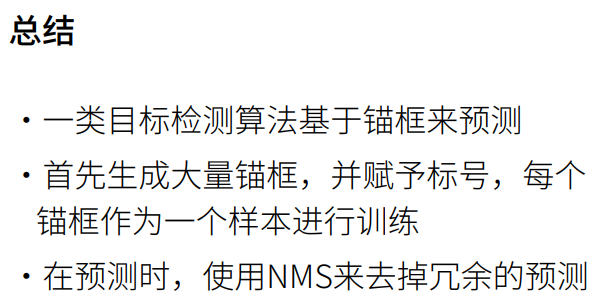
tensor([0, 1, 2, ..., 7, 8, 9])① 锚框的宽度和高度分别是和。我们只考虑组合:
② s表示锚框的大小,锚框占图片的百分之多少,r表示锚框的高宽比。
整体流程总概括(从头到尾干了啥)
- 拿到特征图 H、W、设备信息,计算单个像素锚框个数
- 算出特征图上所有像素归一化中心点坐标
- 根据 sizes、ratios 算出每种锚框对应的归一化宽、高
- 算出每个锚框相对中心的上下左右偏移
- 给每个像素中心点复制多份,匹配对应锚框偏移
- 中心坐标 + 偏移 = 所有锚框的左上角、右下角归一化坐标
- 扩充 batch 维度返回,给后续目标检测匹配真实框、计算损失使用
python
def multibox_prior(data,sizes,ratios):
    """生成以每个像素为中心具有不同高宽度的锚框"""
    # data.shape的最后两个元素为宽和高,第一个元素为通道数
    in_height, in_width = data.shape[-2:]
    # 数据对应的设备、锚框占比个数、锚框高宽比个数
    device, num_sizes, num_ratios = data.device, len(sizes), len(ratios)
    # 计算每个像素点对应的锚框数量
    boxes_per_pixel = (num_sizes + num_ratios - 1)
    # 将锚框占比列表转为张量并将其移动到指定设备
    size_tensor = torch.tensor(sizes, device=device)
    # 将宽高比列表转为张量并将其移动到指定设备
    ratio_tensor = torch.tensor(ratios, device=device)

    # 定义锚框中心偏移量
    offset_h, offset_w = 0.5, 0.5
    # 计算高度方向上的步长
    steps_h = 1.0 / in_height
    # 计算宽度方向上的步长
    steps_w = 1.0 / in_width

    # torch.arange(in_height, device=device)获得每一行像素
    # (torch.arange(in_height, device=device) + offset_h) 获得每一行像素的中心
    # (torch.arange(in_height, device=device) + offset_h) * steps_h 对每一行像素的中心坐标作归一化处理

    # 生成归一化的高度和宽度方向上的像素点中心坐标
    center_h = (torch.arange(in_height, device=device) + offset_h) * steps_h
    center_w = (torch.arange(in_width, device=device) + offset_w) * steps_w
    # 生成坐标网格
    shift_y, shift_x = torch.meshgrid(center_h, center_w)
    # 将坐标网格平铺为一维
    shift_y, shift_x = shift_y.reshape(-1), shift_x.reshape(-1)

    # 计算每个锚框的宽度和高度
    w = torch.cat((size_tensor * torch.sqrt(ratio_tensor[0]),
                  sizes[0] * torch.sqrt(ratio_tensor[1:]))) \
                    * in_height / in_width
    h = torch.cat((size_tensor / torch.sqrt(ratio_tensor[0]),
                  sizes[0] / torch.sqrt(ratio_tensor[1:])))

    # 计算锚框的左上角和右下角坐标(相对于锚框中心的偏移量)
    anchor_manipulations = torch.stack((-w, -h, w, h)).T.repeat(in_height * in_width, 1) / 2

    # 计算所有锚框的中心坐标,每个像素对应boxes_per_pixel个锚框
    out_grid = torch.stack([shift_x, shift_y, shift_x, shift_y], dim=1).repeat_interleave(boxes_per_pixel, dim=0)

    # 通过中心坐标和偏移量计算所有锚框的左上角和右下角坐标
    output = out_grid + anchor_manipulations

    # 增加一个维度并返回结果
    return output.unsqueeze(0)
- 读取一张猫狗图片,拿到图片高、宽像素尺寸
- 构造一个和图片同分辨率的虚拟张量,用来给锚框函数提供尺寸参数
- 设置 3 种缩放尺度、3 种长宽比,调用
multibox_prior为每一个像素中心生成 5 个锚框- 输出所有锚框的整体张量形状,直观验证锚框总数量是否符合计算预期
python
# 返回锚框变量Y的形状
img = d2l.plt.imread('01_Data/img/catdog.jpg')
print("img.shape:",img.shape) # 高561,宽72,3通道
h, w = img.shape[:2]
print(h,w)

X = torch.rand(size=(1,3,h,w)) # 批量大小为1,3通道
Y = multibox_prior(X, sizes=[0.75,0.5,0.25], ratios=[1,2,0.5]) # 占图片sizes尺寸的大小、高宽比ratios尺寸大小的锚框
print(Y.shape) # 1 是批量大小,2042040是一张图片生成的锚框数量,4个元素时每个锚框对应的位置img.shape: (561, 728, 3)
561 728
torch.Size([1, 2042040, 4])
python
# 访问以(250,250)为中心的第一个锚框
boxes = Y.reshape(h,w,5,4)  # 上面的sizes×sizes=3×3,3+3-1=5,故每个像素为中心生成五个锚框
boxes[250,250,0,:] # 以250×250为中心的第一个锚框的坐标tensor([0.06, 0.07, 0.63, 0.82])整体作用:
- 定义通用函数
show_bboxes:在图片画布上批量绘制锚框 / 真实目标框,附带文字标签- 选取坐标
(250,250)像素点对应的全部 5 个锚框,把归一化坐标还原成像素坐标,画在原图上直观查看锚框大小与形态if labels and len(labels) > i:
- 判断当前锚框是否配有标签,有就绘制文字
- 文字颜色自适应:如果框是白色,文字用黑色;其余情况文字白色,保证看得清
rect.xy[0], rect.xy[1]:矩形左上角坐标va='center', ha='center':文字居中摆放- 外层小色块背景和锚框同色,
lw=0去掉边框总结
show_bboxes:通用边界框绘图工具,输入画布、一批框坐标、可选标签、可选颜色,自动批量画框 + 打标注。
python
# 显示以图像中一个像素为中心的所有锚框
def show_bboxes(axes, bboxes, labels=None, colors=None):
    """显示所有边界框"""
    def _make_list(obj, default_values=None):
        # 如果obj为None,使用默认值;如果obj不是列表或元组,将其转换为列表
        if obj is None:
            obj = default_values
        elif not isinstance(obj, (list, tuple)):
            obj = [obj]
        return obj

    # 处理labels,确保其为列表形式
    labels = _make_list(labels)
    # 处理colors,确保其为列表形式
#绘图颜色,不传则默认五色循环:蓝、绿、红、品红、青
    colors = _make_list(colors, ['b','g','r','m','c'])
    # 遍历所有边界框
    for i, bbox in enumerate(bboxes):
        # 选择颜色
        color = colors[i % len(colors)]
        # 使用边界框和颜色生成矩形框
        rect = d2l.bbox_to_rect(bbox.detach().numpy(),color)
        # 在图像上添加矩形框
        axes.add_patch(rect)
        # 如果存在标签
        if labels and len(labels) > i:
            # 根据边界框的颜色选择标签的颜色
            text_color = 'k' if color == 'w' else 'w'
            # 在边界框上添加标签
            axes.text(rect.xy[0], rect.xy[1], labels[i], va='center',
                     ha='center', fontsize=9, color=text_color,
                     bbox=dict(facecolor=color, lw=0))

# 设置图像大小
d2l.set_figsize()
# 创建一个张量来缩放边界框的尺寸
bbox_scale = torch.tensor((w,h,w,h))
# 在图像上显示图像
fig = d2l.plt.imshow(img)
print("fig.axes:",fig.axes)
# 在生成锚框的时候是0-1的值,进行缩放的话就可以省点乘法运算,因为最后输出并不需要显示所有锚框,所以可能会更快一点
print("boxes[250,250,:,:]:",boxes[250,250,:,:])
print("bbox_scale:", bbox_scale)
print("boxes[250,250,:,:] * bbox_scale:",boxes[250,250,:,:] * bbox_scale)
show_bboxes(fig.axes, boxes[250,250,:,:] * bbox_scale, ['s=0.75, r=1','s=0.5, r=1','s=0.25, r=1','s=0.75,r=2','s=0.75,r=0.5']) # 画出以250×250像素为中心的不同高宽比的五个锚框 fig.axes: AxesSubplot(0.125,0.125;0.775x0.755)
boxes[250,250,:,:]: tensor([[ 0.06, 0.07, 0.63, 0.82],
[ 0.15, 0.20, 0.54, 0.70],
[ 0.25, 0.32, 0.44, 0.57],
[-0.06, 0.18, 0.75, 0.71],
[ 0.14, -0.08, 0.55, 0.98]])
bbox_scale: tensor([728, 561, 728, 561])
boxes[250,250,:,:] * bbox_scale: tensor([[ 40.13, 40.12, 460.88, 460.87],
[110.25, 110.25, 390.75, 390.75],
[180.38, 180.38, 320.62, 320.62],
[-47.02, 101.74, 548.02, 399.26],
[101.74, -47.02, 399.26, 548.02]])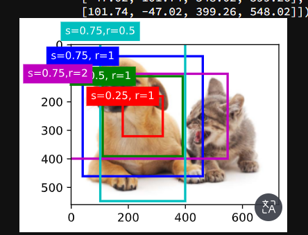
python
# 交并比(IoU)
def box_iou(boxes1,boxes2):
    """计算两个锚框或边界框列表中成对的交并比"""
    # 定义一个lambda函数,计算一个锚框或边界框的面积
    box_area = lambda boxes: ((boxes[:,2] - boxes[:,0]) *
                             (boxes[:,3] - boxes[:,1]))
    # 计算boxes1中每个框的面积
    areas1 = box_area(boxes1)
    # 计算boxes2中每个框的面积
    areas2 = box_area(boxes2)
    # 计算交集区域的左上角坐标(对于每对框,取其左上角坐标的最大值)
    inter_upperlefts = torch.max(boxes1[:,None,:2],boxes2[:,:2])
    # 计算交集区域的右下角坐标(对于每对框,取其右下角坐标的最小值)
    inter_lowerrights = torch.min(boxes1[:,None,2:],boxes2[:,2:])
    # 计算交集区域的宽和高(如果交集不存在,宽和高为0)
    inters = (inter_lowerrights - inter_upperlefts).clamp(min=0)
    # 计算交集区域的面积
    inter_areas = inters[:,:,0] * inters[:,:,1]
    # 计算并集区域的面积(boxes1的面积 + boxes2的面积 - 交集的面积)
    union_areas = areas1[:,None] + areas2 - inter_areas
    # 返回交并比(交集的面积除以并集的面积)
    return inter_areas / union_areas
python
# 将真实边界框分配给锚框
def assign_anchor_to_bbox(ground_truth,anchors,device,iou_threshold=0.5):
    """将最接近的真实边界框分配给锚框"""

    # 获取锚框和真实边界框的数量
    num_anchors, num_gt_boxes = anchors.shape[0], ground_truth.shape[0]

    # 计算所有的锚框和真实边缘框的IOU
    jaccard = box_iou(anchors,ground_truth)

    # 创建一个长度为num_anchors的张量,用-1填充,表示锚框到真实边界框的映射(初始时没有分配)
    anchors_bbox_map = torch.full((num_anchors,), -1, dtype=torch.long, device=device)

    # 对于每个锚框,找到与其IoU最大的真实边界框
    max_ious, indices = torch.max(jaccard, dim=1)

    # 找到IoU大于等于阈值(如0.5)的锚框,将这些锚框分配给对应的真实边界框
    anc_i = torch.nonzero(max_ious >= 0.5).reshape(-1)
    box_j = indices[max_ious >= 0.5]
    anchors_bbox_map[anc_i] = box_j

    # 初始化用于删除行和列的张量
    col_discard = torch.full((num_anchors,),-1)
    row_discard = torch.full((num_gt_boxes,),-1)

    # 通过迭代找到IoU最大的锚框,并将其分配给对应的真实边界框
    for _ in range(num_gt_boxes):
        max_idx = torch.argmax(jaccard) # 找IOU最大的锚框
        box_idx = (max_idx % num_gt_boxes).long() # 通过取余数操作,得到该元素对应的真实边界框的索引
        anc_idx = (max_idx / num_gt_boxes).long() # 通过整除操作,得到该元素对应的锚框的索引

        # 更新锚框到真实边界框的映射
        anchors_bbox_map[anc_idx] = box_idx

        # 在jaccard矩阵中删除已分配的锚框所在的行和列,以避免重复分配
        jaccard[:,box_idx] = col_discard # 把最大Iou对应的锚框在 锚框-类别 矩阵中的一列删掉
        jaccard[anc_idx,:] = row_discard # 把最大Iou对应的锚框在 锚框-类别 矩阵中的一行删掉

    #函数返回一个张量anchors_bbox_map,它的长度与锚框的数量相同。
    #这个张量用于存储每个锚框分配到的真实边界框的索引。
    #如果某个锚框没有分配到真实边界框,那么在这个张量中对应的位置就会是-1。
    #如果某个锚框分配到了真实边界框,那么在这个张量中对应的位置就会是分配到的真实边界框的索引。
    #例如,如果我们有5个锚框和3个真实边界框,那么anchors_bbox_map可能会是这样的:[0, -1, 1, 2, -1]。这表示第1个锚框被分配到了第1个真实边界框,第2个锚框没有被分配到真实边界框,第3个锚框被分配到了第2个真实边界框,第4个锚框被分配到了第3个真实边界框,第5个锚框没有被分配到真实边界框。
    return anchors_bbox_map
③ 给定框A和B,中心坐标分别为和,宽度分别为和,高度分别为和。
④ 我们可以将A的偏移量标记为
python
def offset_boxes(anchors,assigned_bb,eps=1e-6):
    """对锚框偏移量的转换"""
    # 将锚框从(左上角, 右下角)的形式转换为(中心点, 宽度, 高度)的形式
    c_anc = d2l.box_corner_to_center(anchors)
    # 将被分配的真实边界框从(左上角, 右下角)的形式转换为(中心点, 宽度, 高度)的形式
    c_assigned_bb = d2l.box_corner_to_center(assigned_bb)
    # 计算中心点的偏移量,并进行缩放
    offset_xy = 10 * (c_assigned_bb[:,:2] - c_anc[:,:2] / c_anc[:,2:])
    # 计算宽度和高度的偏移量,并进行缩放
    offset_wh = 5 * torch.log(eps + c_assigned_bb[:,2:] / c_anc[:,2:])
    # 将中心点和宽高的偏移量合并在一起
    offset = torch.cat([offset_xy, offset_wh], axis=1)
    # 返回计算得到的偏移量
    return offset
python
# 标记锚框的类和偏移量
def multibox_target(anchors, labels):
    """使用真实边界框标记锚框"""
    # 获取批量大小和锚框
    batch_size, anchors = labels.shape[0], anchors.squeeze(0)
    # 初始化偏移量、掩码和类别标签列表
    batch_offset, batch_mask, batch_class_labels = [], [], []
    # 获取设备和锚框数量
    device, num_anchors = anchors.device, anchors.shape[0]
    # 对于每个样本
    for i in range(batch_size):
        # 获取该样本的标签
        label = labels[i,:,:]
        # 将最接近的真实边界框分配给锚框
        anchors_bbox_map = assign_anchor_to_bbox(label[:,1:],anchors,device)
        # 生成锚框掩码,用于标记哪些锚框包含目标
        bbox_mask = ((anchors_bbox_map >= 0).float().unsqueeze(-1)).repeat(1,4)
        # 初始化类别标签
        class_labels = torch.zeros(num_anchors, dtype=torch.long,device=device)
        # 初始化被分配的边界框
        assigned_bb = torch.zeros((num_anchors,4), dtype=torch.float32,device=device)
        # 获取包含目标的锚框的索引
        indices_true =torch.nonzero(anchors_bbox_map >= 0)
        # 获取对应的真实边界框的索引
        bb_idx = anchors_bbox_map[indices_true]
        # 设置包含目标的锚框的类别标签
        class_labels[indices_true] = label[bb_idx,0].long() + 1
        # 设置被分配的边界框
        assigned_bb[indices_true] = label[bb_idx, 1:]
        # 计算锚框的偏移量,并通过掩码进行过滤
        offset = offset_boxes(anchors, assigned_bb) * bbox_mask
        # 将偏移量添加到列表中
        batch_offset.append(offset.reshape(-1))
        # 将掩码添加到列表中
        batch_mask.append(bbox_mask.reshape(-1))
        # 将类别标签添加到列表中
        batch_class_labels.append(class_labels)
    # 将所有偏移量堆叠在一起
    bbox_offset = torch.stack(batch_offset)
    # 将所有掩码堆叠在一起
    bbox_mask = torch.stack(batch_mask)
    # 将所有类别标签堆叠在一起
    class_labels = torch.stack(batch_class_labels)
    # 返回每一个锚框到真实标注框的offset偏移
    # bbox_mask为0表示背景锚框,就不用了,为1表示对应真实的物体
    # class_labels为锚框对应类的编号
    # 返回偏移量、掩码和类别标签
    return (bbox_offset, bbox_mask, class_labels)
python
# 在图像中绘制这些地面真相边界框和锚框

# 两个真实边缘框的位置信息
ground_truth = torch.tensor([[0,0.1,0.08,0.52,0.92],
                            [1,0.55,0.2,0.9,0.88]]) # 真实标注框的信息,包括类别标签(0代表狗,1代表猫)和位置信息(归一化的坐标)

# 五个锚框的位置信息
anchors = torch.tensor([[0,0.1,0.2,0.3],[0.15,0.2,0.4,0.4],
                       [0.63,0.05,0.88,0.98],[0.66,0.45,0.8,0.8],
                       [0.57,0.3,0.92,0.9]]) # 锚框的位置信息(归一化的坐标)

fig = d2l.plt.imshow(img)
# 在图像上画出真实的边界框,其中'k'代表黑色
show_bboxes(fig.axes,ground_truth[:,1:] * bbox_scale, ['dog','cat'],'k')
# 在图像上画出锚框,标注出锚框的索引号
show_bboxes(fig.axes,anchors * bbox_scale, ['0','1','2','3','4']) 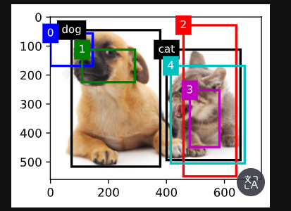
python
# 根据狗和猫的真实边界框,标注这些锚框的分类和偏移量

# anchors.unsqueeze(dim=0)在0号位置加了一个批量维度,该批量维度大小为1
labels = multibox_target(anchors.unsqueeze(dim=0),ground_truth.unsqueeze(dim=0))
# labels 对应 multibox_target 函数返回的  (bbox_offset, bbox_mask, class_labels)
print(len(labels))
# labels[2]有五个锚框 0表示背景、1表示狗、2表示猫 这里3号框被表示为背景是因为被2号框和四号框非极大值抑制了
print(labels[2])
# 锚框是不是对应是真实物体
print(labels[1])
# 每一个锚框有四个值,0表示不需要预测,
print(labels[0]) 3
tensor([[0, 1, 2, 0, 2]])
tensor([[0., 0., 0., 0., 1., 1., 1., 1., 1., 1., 1., 1., 0., 0., 0., 0., 1., 1.,
1., 1.]])
tensor([[-0.00e+00, -0.00e+00, -0.00e+00, -0.00e+00, -7.90e+00, -1.00e+01,
2.59e+00, 7.18e+00, -2.30e+01, -1.38e-01, 1.68e+00, -1.57e+00,
-0.00e+00, -0.00e+00, -0.00e+00, -0.00e+00, -1.40e+01, -4.60e+00,
4.17e-06, 6.26e-01]])
python
# 应用逆偏移变换来返回预测的边界框坐标
def offset_inverse(anchors,offset_preds):
    """根据带有预测偏移量的锚框来预测边界框"""
    # 将锚框从角点表示转换为中心-宽度表示
    anc = d2l.box_corner_to_center(anchors)
    # 利用预测的偏移量和原始锚框,计算预测边界框的中心坐标
    pred_bbox_xy = (offset_preds[:,:2] * anc[:,2:] / 10) + anc[:,:2]
    # 利用预测的偏移量和原始锚框,计算预测边界框的宽度和高度
    pred_bbox_wh = torch.exp(offset_preds[:,2:] / 5) * anc[:, 2:]
    # 将预测边界框的中心坐标和宽高组合在一起,得到预测边界框的中心-宽度表示
    pred_bbox = torch.cat((pred_bbox_xy, pred_bbox_wh), axis=1)
    # 将预测边界框从中心-宽度表示转换为角点表示
    predicted_bbox = d2l.box_center_to_corner(pred_bbox)
    # 返回预测的边界框
    return predicted_bbox # 将锚框用偏移量进行偏移,得到预测的边界框
python
# 以下nms函数按降序对置信度进行排序并返回其索引
def nms(boxes, scores, iou_threshold):
    """对预测边界框的置信度进行排序"""
    # 按照得分降序排列预测边界框的索引
    B = torch.argsort(scores, dim = -1, descending=True)
    # 创建一个空列表,用于存储保留下来的边界框索引
    keep = []
    # 当B中还有元素时,进行循环
    while B.numel()>0: # 直到把所有框都访问过了,再退出循环
        # 取B中得分最高的边界框索引
        i = B[0] # B中的最大值,已经排好序了
        # 将这个边界框索引添加到保留列表中
        keep.append(i)
        # 如果B中只有一个元素,那么结束循环
        if B.numel() == 1: break
        # 计算剩余的边界框与当前得分最高的边界框的IoU(交并比)
        iou = box_iou(boxes[i,:].reshape(-1,4),
                     boxes[B[1:],:].reshape(-1,4)).reshape(-1)
        # 找到所有与当前得分最高的边界框的IoU不大于阈值的边界框的索引
        inds = torch.nonzero(iou <= iou_threshold).reshape(-1)
        # 保留那些与当前得分最高的边界框的IoU不大于阈值的边界框
        B = B[inds + 1]
    # 返回保留下来的边界框索引
    return torch.tensor(keep, device=boxes.device)
python
# 将非极大值抑制应用于预测边界框
def multibox_detection(cls_probs,offset_preds,anchors,nms_threshold=0.5,
                      pos_threshold=0.009999999):
    """使用非极大值抑制来预测边界框"""
    # 获取设备类型和批次大小
    device, batch_size = cls_probs.device, cls_probs.shape[0]
    # 将锚框数据压缩到二维
    anchors = anchors.squeeze(0)
    # 获取类别数量和锚框数量
    num_classes, num_anchors = cls_probs.shape[1], cls_probs.shape[2]
    # 创建一个空列表,用于存储每个批次的预测结果
    out = []
    # 对每个批次进行循环
    for i in range(batch_size):

        # 获取类别概率和预测的偏移量
        cls_prob, offset_pred = cls_probs[i], offset_preds[i].reshape(-1,4)

        # 获取最大类别概率和对应的类别id
        conf, class_id = torch.max(cls_prob[1:],0)

        # 根据预测的偏移量和锚框得到预测的边界框
        predicted_bb = offset_inverse(anchors,offset_pred) # 把预测框拿出来

        # 对预测的边界框进行非极大值抑制,获取保留下来的边界框索引
        keep = nms(predicted_bb, conf, nms_threshold)

        # 获取所有的边界框索引
        all_idx = torch.arange(num_anchors, dtype=torch.long, device=device)

        # 将保留下来的边界框索引和所有的边界框索引拼接在一起
        combined = torch.cat((keep,all_idx))

        # 获取唯一的索引和对应的计数
        uniques, counts = combined.unique(return_counts=True)

        # 获取被丢弃的边界框索引
        non_keep = uniques[counts==1]

        # 将保留下来的边界框索引和被丢弃的边界框索引按顺序拼接在一起
        all_id_sorted = torch.cat((keep, non_keep))

        # 将被丢弃的边界框的类别id设为-1
        class_id[non_keep] = -1
        class_id = class_id[all_id_sorted]

        # 根据索引获取对应的类别概率和预测的边界框
        conf, predicted_bb = conf[all_id_sorted], predicted_bb[all_id_sorted]

        # 找到类别概率低于阈值的边界框索引
        below_min_idx = (conf < pos_threshold)

        # 将类别概率低于阈值的边界框的类别id设为-1
        class_id[below_min_idx] = -1

        # 将类别概率低于阈值的边界框的类别概率设为1减去原来的值
        conf[below_min_idx] = 1 - conf[below_min_idx]

        # 将类别id,类别概率和预测的边界框拼接在一起,作为预测信息
        pred_info = torch.cat((class_id.unsqueeze(1),conf.unsqueeze(1),predicted_bb),dim=1)

        # 将每个批次的预测信息添加到结果列表中
        out.append(pred_info)

    # 将结果列表转为张量返回
    return torch.stack(out)
python
# 将上述算法应用到一个带有四个锚框的具体示例中

# 四个锚框的坐标
anchors = torch.tensor([[0.1,0.08,0.52,0.92],[0.08,0.2,0.56,0.95],
                       [0.15,0.3,0.62,0.91],[0.55,0.2,0.9,0.88]])

# 偏移预测值,这里假设预测值全为0,即没有预测偏移
offset_preds = torch.tensor([0] * anchors.numel())
print("offset_preds:", offset_preds) # 打印偏移预测值
print("len(offset_preds):", len(offset_preds)) # 打印偏移预测值的长度

# 类别概率,每一列对应一个锚框,每一行对应一个类别,这里有三个类别:背景、猫、狗
cls_probs = torch.tensor([[0] * 4,  # 背景类别概率
                         [0.9, 0.8, 0.7, 0.1],  # 猫类别概率
                         [0.1, 0.2, 0.3, 0.9]]) # 狗类别概率
print("cls_probs:", cls_probs) # 四个锚框对背景、猫、狗这三个类的预测值,每一列为一个锚框 offset_preds: tensor([0, 0, 0, 0, 0, 0, 0, 0, 0, 0, 0, 0, 0, 0, 0, 0])
len(offset_preds): 16
cls_probs: tensor([[0.00, 0.00, 0.00, 0.00],
[0.90, 0.80, 0.70, 0.10],
[0.10, 0.20, 0.30, 0.90]])
python
# 在图像上绘制这些预测边界框和置信度
# 创建一个图像对象,并在图像上显示
fig = d2l.plt.imshow(img)
# 在图像上显示锚框,其中锚框的尺度需要进行转换以适应图像的尺度
# 每个锚框旁边的文本表示该锚框预测为某个类别的置信度
show_bboxes(fig.axes, anchors * bbox_scale, # 没有做NMS时,把四个锚框画出来
           ['dog=0.9','dog=0.8','dog=0.7','cat=0.9'])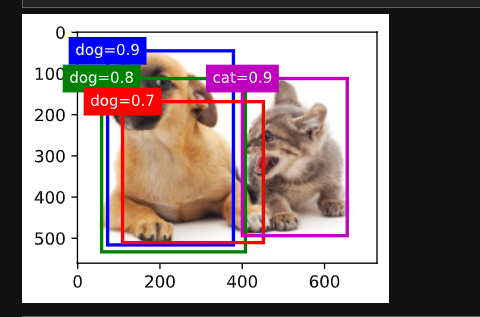
python
# 使用multibox_detection函数,输入类别预测概率、预测偏移量以及锚框,同时设置非极大值抑制的阈值为0.5
# 注意,这里需要先在输入数据的每个维度上添加一个维度(即批量大小的维度),然后才能传入函数
output = multibox_detection(cls_probs.unsqueeze(dim=0),
                           offset_preds.unsqueeze(dim=0),
                           anchors.unsqueeze(dim=0),nms_threshold=0.5)
# 打印输出结果,这里的输出结果包含了每个锚框的类别预测、置信度以及经过预测偏移调整后的锚框坐标
# output[0]表示批量中的第一张图片的预测结果
print("output:",output) #output[0]为批量大小中的第一个图片output: tensor([[[ 0.00, 0.90, 0.10, 0.08, 0.52, 0.92],
[ 1.00, 0.90, 0.55, 0.20, 0.90, 0.88],
[-1.00, 0.80, 0.08, 0.20, 0.56, 0.95],
[-1.00, 0.70, 0.15, 0.30, 0.62, 0.91]]])
python
# 输出由非极大值抑制保存的最终预测边界框

# 在图像上绘制通过非极大值抑制筛选后的预测边界框
fig = d2l.plt.imshow(img)

# 输出经过非极大值抑制后的预测结果
print("output[0]:", output[0])

# 遍历预测结果
for i in output[0].detach().numpy():

    # 输出当前预测结果的详细信息
    print(i)

    # 判断如果预测结果的类别为-1,说明这个预测结果表示的是背景或在非极大值抑制中被移除了,所以我们直接跳过这个结果
    if i[0] == -1: # 值-1表示背景或在非极大值抑制中被移除了
        continue

    # 打印预测的类别和置信度
    print("int(i[0]):", int(i[0]))  # i[0]=0表示狗,i[0]=1表示猫,即i的第一个元素表示框对应的类别
    print("str(i[1]):", str(i[1]))  # i的第二元素表示该类别的置信度

    # 根据预测的类别和置信度生成标签
    label = ('dog=', 'cat=')[int(i[0])] + str(i[1]) # 取('dog=', 'cat=')元组的第int(i[0]位置与str(i[1])进行拼接
    print("label:",label)

    # 在图像上绘制预测的边界框和标签
show_bboxes(fig.axes, [torch.tensor(i[2:]) * bbox_scale], label)output[0]: tensor([[ 0.00, 0.90, 0.10, 0.08, 0.52, 0.92],
[ 1.00, 0.90, 0.55, 0.20, 0.90, 0.88],
[-1.00, 0.80, 0.08, 0.20, 0.56, 0.95],
[-1.00, 0.70, 0.15, 0.30, 0.62, 0.91]])
[0. 0.9 0.10000001 0.07999998 0.52 0.92 ]
int(i[0]): 0
str(i[1]): 0.9
label: dog=0.9
[1. 0.9 0.5500001 0.20000002 0.9 0.88 ]
int(i[0]): 1
str(i[1]): 0.9
label: cat=0.9
[-1. 0.8 0.07999998 0.19999999 0.56 0.95 ]
[-1. 0.7 0.14999999 0.3 0.62 0.91 ]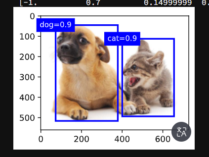
7. 树叶分类竞赛技术总结

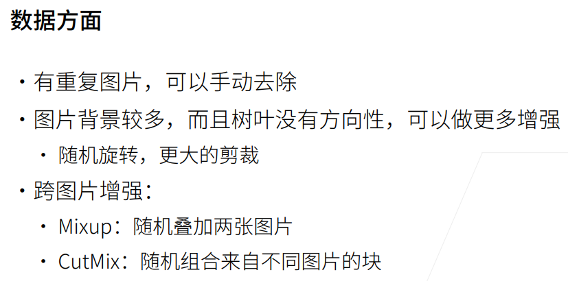
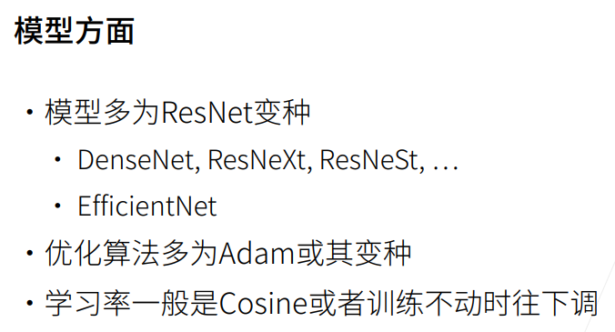

1. 总结