LeNet-5 详解：从一只猫的图片看懂卷积神经网络的经典架构

1998 年，Yann LeCun 等人提出了 LeNet-5 网络，用于手写数字识别。它虽然结构简单，却完整定义了**卷积-池化-全连接**的基本范式，是现代 CNN 的鼻祖。

本 notebook 使用 PyTorch 从零复现 LeNet-5，用一张32×32 的猫咪灰度照片，一步步追踪它在网络中的完整数据变换。每一层的尺寸、计算和特征图可视化都清晰展示。

import torch
import torch.nn as nn
import torch.nn.functional as F
from torchvision import transforms
from PIL import Image
import numpy as np
import matplotlib.pyplot as plt
import matplotlib

# 配置中文字体
plt.rcParams['font.sans-serif'] = ['SimHei', 'Microsoft YaHei', 'DejaVu Sans']
plt.rcParams['axes.unicode_minus'] = False

# 固定随机种子，保证结果可复现
torch.manual_seed(42)
np.random.seed(42)

print("所有库导入成功！PyTorch 版本:", torch.__version__)

1. 准备猫咪图片：输入层

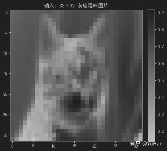
我们有一张正方形的猫咪照片，下面将它缩放为 32×32 像素 的灰度图，像素值归一化到 0 到 1 之间。

数据形态 ：1@32×32 （1 个通道，高 32，宽 32）

# 预处理：转灰度 → 缩放到 32×32 → 归一化到 [0,1]
transform = transforms.Compose([
    transforms.Grayscale(num_output_channels=1),
    transforms.Resize((32, 32)),
    transforms.ToTensor(),
])

image_pil = Image.open('image/cat.10006.jpg')
input_tensor = transform(image_pil).unsqueeze(0)  # 增加 batch 维度: (1, 1, 32, 32)

print(f"输入张量形状: {input_tensor.shape}  (batch, channel, height, width)")
print(f"数值范围: [{input_tensor.min():.4f}, {input_tensor.max():.4f}]")
输入张量形状: torch.Size([1, 1, 32, 32])  (batch, channel, height, width)
数值范围: [0.1373, 0.9176]

我们将input_tensor转换成图片看看结果

# 显示输入图片
plt.figure(figsize=(6, 6))
plt.imshow(input_tensor.squeeze().numpy(), cmap='gray')
plt.title('输入：32×32 灰度猫咪图片')
plt.colorbar(fraction=0.046, pad=0.04)
plt.show()

# 打印左上角 5×5 区域
print("\n左上角 5×5 区域像素值（归一化）:")
print(input_tensor.squeeze().numpy()[:5, :5].round(2))

左上角 5×5 区域像素值（归一化）:
[[0.58 0.6  0.61 0.62 0.64]
 [0.59 0.6  0.62 0.63 0.64]
 [0.6  0.62 0.62 0.64 0.64]
 [0.6  0.62 0.63 0.64 0.64]
 [0.61 0.63 0.64 0.65 0.65]]

运行结果如下：

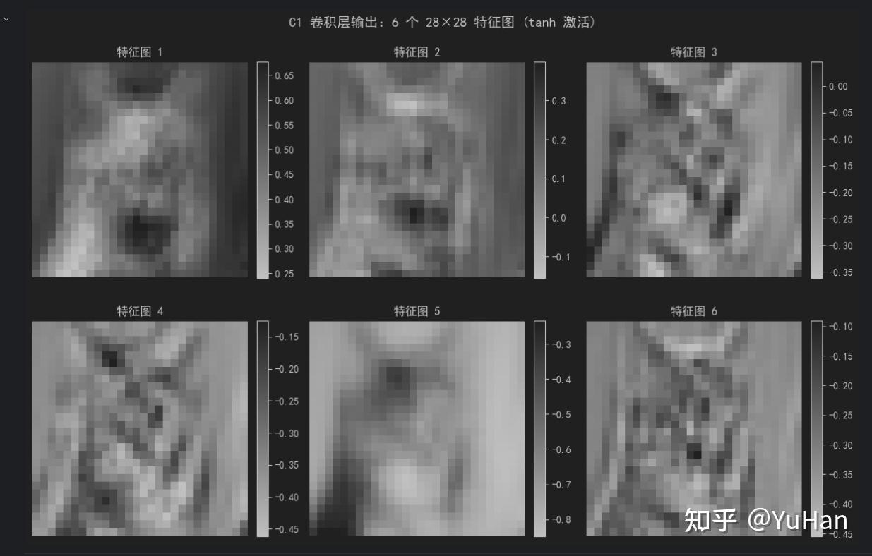
2. 第一层 C1：卷积层

操作说明

• 输入 ：32×32×1
• 卷积核 ：6 个，每个尺寸 5×5，步长 = 1，不填充（valid 卷积）
• 输出尺寸计算 ：(32 - 5)/1 + 1 = 28，即 6 张 28×28 的特征图
• 激活函数 ：tanh
• 参数量 ：每个卷积核有 5×5 = 25 个权重，再加 1 个偏置，共 26 个参数。6 个卷积核总计 6×26 = 156 个参数。

数据变换 ：1@32×32 → 6@28×28

# 定义 C1 卷积层
c1 = nn.Conv2d(in_channels=1, out_channels=6, kernel_size=5, stride=1, padding=0)
print(f"C1 参数量: {sum(p.numel() for p in c1.parameters())} 个")
print(f"卷积核形状: {c1.weight.shape}  (out_channels, in_channels, kernel_h, kernel_w)")

# 前向传播 + tanh 激活
with torch.no_grad():
    c1_output = torch.tanh(c1(input_tensor))

print(f"\n输入尺寸: {input_tensor.shape}")
print(f"C1 输出尺寸: {c1_output.shape}")
print(f"输出数值范围: [{c1_output.min():.4f}, {c1_output.max():.4f}] (tanh 激活后在 -1 到 1 之间)")

# 可视化 6 个特征图
fig, axes = plt.subplots(2, 3, figsize=(12, 8))
fig.suptitle('C1 卷积层输出：6 个 28×28 特征图 (tanh 激活)', fontsize=14)
for i in range(6):
    ax = axes[i // 3, i % 3]
    im = ax.imshow(c1_output.squeeze()[i].numpy(), cmap='gray')
    ax.set_title(f'特征图 {i+1}')
    ax.axis('off')
    plt.colorbar(im, ax=ax, fraction=0.046, pad=0.04)
plt.tight_layout()
plt.show()

# 展示第一个卷积核的权重
print("\n第一个卷积核的权重 (5×5):")
print(c1.weight[0, 0].detach().numpy().round(3))
C1 参数量: 156 个
卷积核形状: torch.Size([6, 1, 5, 5])  (out_channels, in_channels, kernel_h, kernel_w)

输入尺寸: torch.Size([1, 1, 32, 32])
C1 输出尺寸: torch.Size([1, 6, 28, 28])
输出数值范围: [-0.8493, 0.6776] (tanh 激活后在 -1 到 1 之间)

第一个卷积核的权重 (5×5):
[[ 0.153  0.166 -0.047  0.184 -0.044]
 [ 0.04  -0.097  0.117  0.176 -0.147]
 [ 0.174  0.037  0.148  0.027  0.096]
 [-0.028  0.154  0.03  -0.093  0.051]
 [-0.092 -0.023 -0.081  0.133 -0.158]]

6个特征图如下所示：

手动演示卷积计算

为了理解卷积是如何计算的，我们手动用第一个卷积核对输入图片的左上角 5×5 区域做一次卷积：

y = \tanh\left( \sum_{i=0}^{{4}\sum_{j=0}}{4} w_{i,j} \cdot x_{i,j} + b \right)

# 取输入图片左上角 5×5 区域
patch = input_tensor[0, 0, :5, :5].numpy()
kernel = c1.weight[0, 0].detach().numpy()
bias = c1.bias[0].item()

# 手动计算卷积：逐元素相乘求和 + 偏置
conv_sum = np.sum(patch * kernel) + bias
activated = np.tanh(conv_sum)

print("输入区域 (5×5):")
print(patch.round(3))
print("\n卷积核权重 (5×5):")
print(kernel.round(3))
print(f"\n偏置 b = {bias:.4f}")
print(f"逐元素乘积累加 + 偏置 = {conv_sum:.4f}")
print(f"tanh 激活后 = {activated:.4f}")
print(f"\n与 PyTorch 计算结果对比: {c1_output[0, 0, 0, 0].item():.4f}")
print(f"结果一致: {np.isclose(activated, c1_output[0, 0, 0, 0].item())}")
输入区域 (5×5):
[[0.58  0.6   0.612 0.624 0.635]
 [0.592 0.604 0.62  0.631 0.639]
 [0.604 0.62  0.624 0.635 0.643]
 [0.604 0.624 0.631 0.643 0.643]
 [0.608 0.627 0.643 0.647 0.651]]

卷积核权重 (5×5):
[[ 0.153  0.166 -0.047  0.184 -0.044]
 [ 0.04  -0.097  0.117  0.176 -0.147]
 [ 0.174  0.037  0.148  0.027  0.096]
 [-0.028  0.154  0.03  -0.093  0.051]
 [-0.092 -0.023 -0.081  0.133 -0.158]]

偏置 b = 0.0503
逐元素乘积累加 + 偏置 = 0.5823
tanh 激活后 = 0.5243

与 PyTorch 计算结果对比: 0.5243
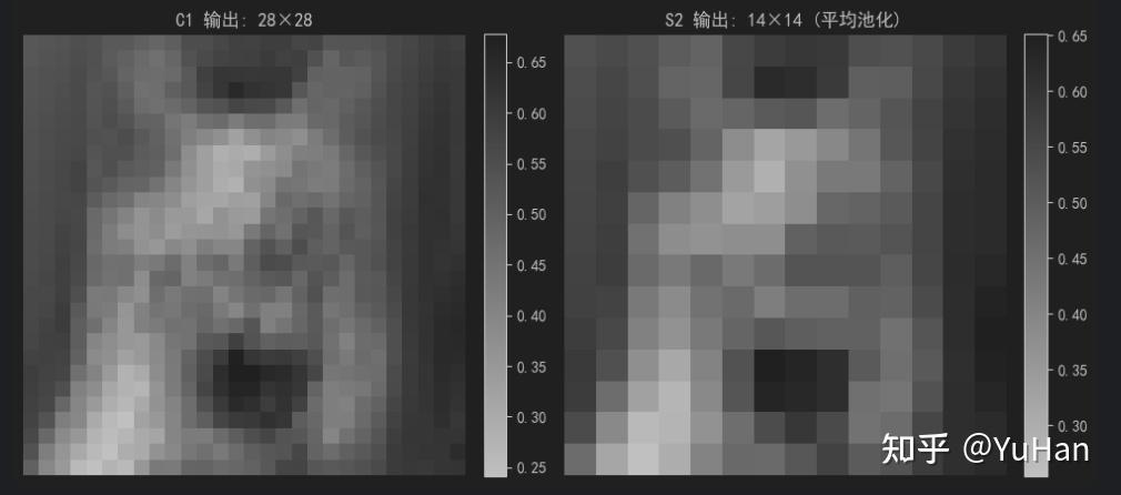
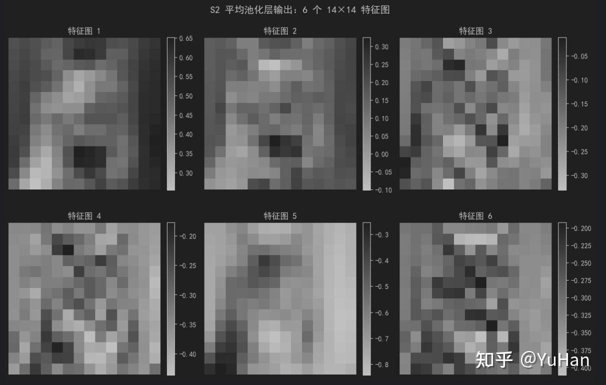
结果一致: True

3. 第二层 S2：平均池化层

操作说明

• 输入 ：6@28×28
• 池化窗口 ：2×2，步长 = 2
• 输出尺寸 ：14×14，通道数保持 6，即 6@14×14

池化的作用：保留主要特征的同时，将数据量减少为原来的 1/4，还能抑制微小位置变化带来的影响。

数据变换 ：6@28×28 → 6@14×14

# 定义平均池化层
s2 = nn.AvgPool2d(kernel_size=2, stride=2)

# 前向传播
with torch.no_grad():
    s2_output = s2(c1_output)

print(f"S2 输入尺寸: {c1_output.shape}")
print(f"S2 输出尺寸: {s2_output.shape}")
print(f"空间尺寸压缩比: ({c1_output.shape[2]}/{s2_output.shape[2]})² = {(c1_output.shape[2]/s2_output.shape[2])**2:.0f} 倍")

# 可视化池化前后对比（取第一个特征图）
fig, axes = plt.subplots(1, 2, figsize=(10, 5))

im0 = axes[0].imshow(c1_output.squeeze()[0].numpy(), cmap='gray')
axes[0].set_title(f'C1 输出: 28×28')
axes[0].axis('off')
plt.colorbar(im0, ax=axes[0], fraction=0.046, pad=0.04)

im1 = axes[1].imshow(s2_output.squeeze()[0].numpy(), cmap='gray')
axes[1].set_title(f'S2 输出: 14×14 (平均池化)')
axes[1].axis('off')
plt.colorbar(im1, ax=axes[1], fraction=0.046, pad=0.04)

plt.tight_layout()
plt.show()

# 手动验证第一个 2×2 区域的平均池化
print("\n=== 手动验证平均池化 ===")
c1_patch = c1_output[0, 0, :2, :2].numpy()
manual_avg = np.mean(c1_patch)
pytorch_val = s2_output[0, 0, 0, 0].item()
print(f"C1 第一个 2×2 区域:\n{c1_patch.round(4)}")
print(f"手动计算平均值: {manual_avg:.6f}")
print(f"PyTorch 输出值: {pytorch_val:.6f}")
print(f"结果一致: {np.isclose(manual_avg, pytorch_val)}")
S2 输入尺寸: torch.Size([1, 6, 28, 28])
S2 输出尺寸: torch.Size([1, 6, 14, 14])
空间尺寸压缩比: (28/14)² = 4 倍

=== 手动验证平均池化 ===
C1 第一个 2×2 区域:
[[0.5243 0.5323]
 [0.5263 0.5375]]
手动计算平均值: 0.530122
PyTorch 输出值: 0.530122
结果一致: True

第一个特征图池化对比

# 显示全部 6 个池化后的特征图
fig, axes = plt.subplots(2, 3, figsize=(12, 8))
fig.suptitle('S2 平均池化层输出：6 个 14×14 特征图', fontsize=14)
for i in range(6):
    ax = axes[i // 3, i % 3]
    im = ax.imshow(s2_output.squeeze()[i].numpy(), cmap='gray')
    ax.set_title(f'特征图 {i+1}')
    ax.axis('off')
    plt.colorbar(im, ax=ax, fraction=0.046, pad=0.04)
plt.tight_layout()
plt.show()

S2 平均池化层输出：6 个 14×14 特征图如下所示：

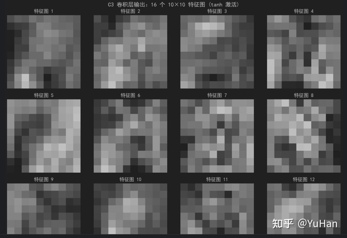
4. 第三层 C3：卷积层（多通道组合）

操作说明

• 输入 ：6@14×14（6 个特征图）
• 卷积核 ：16 组，每组核的尺寸为 5×5，输入有 6 个通道
• 输出尺寸 ：(14 - 5)/1 + 1 = 10，即 16@10×10
• 激活函数 ：tanh

这里每个输出特征图由 6 个 5×5 卷积核分别处理 6 个输入通道，结果相加后加偏置，再经 tanh。网络开始组合出更高级的特征。

数据变换 ：6@14×14 → 16@10×10

# 定义 C3 卷积层
c3 = nn.Conv2d(in_channels=6, out_channels=16, kernel_size=5, stride=1, padding=0)
print(f"C3 参数量: {sum(p.numel() for p in c3.parameters())} 个")
print(f"卷积核形状: {c3.weight.shape}  (out_channels, in_channels, kernel_h, kernel_w)")

# 前向传播 + tanh 激活 
with torch.no_grad():
    c3_output = torch.tanh(c3(s2_output))

print(f"\n输入尺寸: {s2_output.shape}")
print(f"C3 输出尺寸: {c3_output.shape}")

# 可视化 16 个特征图
fig, axes = plt.subplots(4, 4, figsize=(12, 12))
fig.suptitle('C3 卷积层输出：16 个 10×10 特征图 (tanh 激活)', fontsize=14)
for i in range(16):
    ax = axes[i // 4, i % 4]
    im = ax.imshow(c3_output.squeeze()[i].numpy(), cmap='gray')
    ax.set_title(f'特征图 {i+1}')
    ax.axis('off')
plt.tight_layout()
plt.show()
C3 参数量: 2416 个
卷积核形状: torch.Size([16, 6, 5, 5])  (out_channels, in_channels, kernel_h, kernel_w)

输入尺寸: torch.Size([1, 6, 14, 14])
C3 输出尺寸: torch.Size([1, 16, 10, 10])

C3 卷积层输出：16 个 10×10 特征图 (tanh 激活) 图片如下(未截取全）:

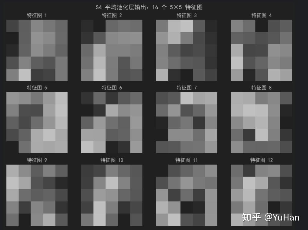
5. 第四层 S4：第二个平均池化层

操作说明

• 输入 ：16@10×10
• 池化窗口 ：2×2，步长 = 2
• 输出尺寸 ：5×5，即 16@5×5

经过这一步，每张特征图只剩下 25 个数值，但每一个都浓缩了较大感受野内的关键信息。

数据变换 ：16@10×10 → 16@5×5

# 定义 S4 平均池化层
s4 = nn.AvgPool2d(kernel_size=2, stride=2)

with torch.no_grad():
    s4_output = s4(c3_output)

print(f"S4 输入尺寸: {c3_output.shape}")
print(f"S4 输出尺寸: {s4_output.shape}")

# 可视化 16 个池化后的特征图
fig, axes = plt.subplots(4, 4, figsize=(10, 10))
fig.suptitle('S4 平均池化层输出：16 个 5×5 特征图', fontsize=14)
for i in range(16):
    ax = axes[i // 4, i % 4]
    im = ax.imshow(s4_output.squeeze()[i].numpy(), cmap='gray')
    ax.set_title(f'特征图 {i+1}')
    ax.axis('off')
plt.tight_layout()
plt.show()

# 打印第一个特征图的 5×5 数值
print("\n第一个特征图的 5×5 像素值:")
print(s4_output.squeeze()[0].numpy().round(4))
S4 输入尺寸: torch.Size([1, 16, 10, 10])
S4 输出尺寸: torch.Size([1, 16, 5, 5])

第一个特征图的 5×5 像素值:
[[0.2778 0.249  0.2063 0.2234 0.2391]
 [0.3161 0.2488 0.1948 0.2037 0.2362]
 [0.3058 0.245  0.1997 0.2177 0.2435]
 [0.2644 0.21   0.2499 0.2599 0.2222]
 [0.2144 0.1456 0.2847 0.2783 0.2203]]

S4 平均池化层输出：16 个 5×5 特征图：

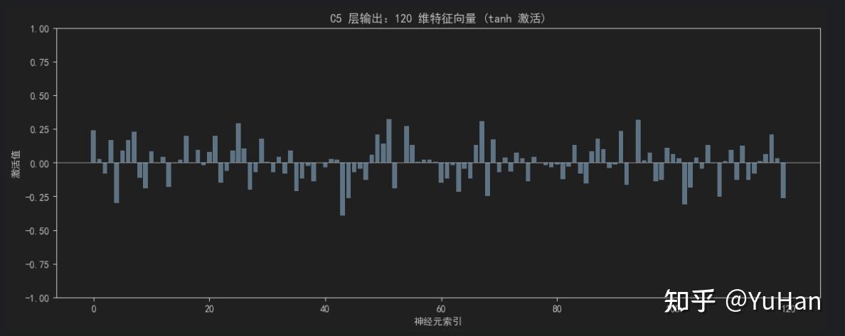
6. 第五层 C5：卷积层（实质为全连接）

操作说明

• 输入 ：16@5×5
• 卷积核 ：120 个，每个尺寸 5×5，与输入图尺寸完全相同
• 输出尺寸 ：(5 - 5)/1 + 1 = 1，即 120 个 1×1 的特征图，可拉直为 120 维向量
• 激活函数 ：tanh
• 参数量 ：(5×5×16 + 1) × 120 = 48120

因为卷积核和输入的空间尺寸一样大，这一步实际上就是全连接。每一个神经元对应一个复杂的视觉概念。

数据变换 ：16@5×5 → 120 维向量

# 定义 C5 卷积层 (kernel_size=5, 输入也是 5×5，输出就是 1×1)
c5 = nn.Conv2d(in_channels=16, out_channels=120, kernel_size=5, stride=1, padding=0)
print(f"C5 参数量: {sum(p.numel() for p in c5.parameters())} 个")
print(f"卷积核形状: {c5.weight.shape}")

with torch.no_grad():
    c5_output = torch.tanh(c5(s4_output))

print(f"\n输入尺寸: {s4_output.shape}")
print(f"C5 输出尺寸: {c5_output.shape}")

# 拉平为向量
c5_flat = c5_output.view(-1)
print(f"拉平后维度: {c5_flat.shape} = 120 维向量")

# 可视化 120 维向量（柱状图）
plt.figure(figsize=(14, 5))
plt.bar(range(120), c5_flat.numpy(), color='steelblue')
plt.title('C5 层输出：120 维特征向量 (tanh 激活)')
plt.xlabel('神经元索引')
plt.ylabel('激活值')
plt.ylim(-1, 1)
plt.axhline(y=0, color='black', linewidth=0.5)
plt.show()

print("\n前 20 个神经元的激活值:")
print(c5_flat[:20].numpy().round(4))
C5 参数量: 48120 个
卷积核形状: torch.Size([120, 16, 5, 5])

输入尺寸: torch.Size([1, 16, 5, 5])
C5 输出尺寸: torch.Size([1, 120, 1, 1])
拉平后维度: torch.Size([120]) = 120 维向量

前 20 个神经元的激活值:
[ 0.2397  0.0268 -0.0841  0.1685 -0.2991  0.0904  0.169   0.2291 -0.1136
 -0.1908  0.0845 -0.0045  0.0436 -0.1811 -0.0047  0.0207  0.1973 -0.0045
  0.093  -0.0199]

C5 层输出：120 维特征向量 (tanh 激活)，使用图表展示：

7. 第六层 F6：全连接层

操作说明

• 输入：120 维向量
• 输出：84 个神经元
• 计算方式 ：标准的全连接，即 输出 = tanh(W·输入 + b)
• 参数量 ：120 × 84 + 84 = 10164

这 84 个神经元可以看作更抽象的"特征编码"。

数据变换 ：120 维 → 84 维

# 定义 F6 全连接层
f6 = nn.Linear(in_features=120, out_features=84)
print(f"F6 参数量: {sum(p.numel() for p in f6.parameters())} 个")

with torch.no_grad():
    f6_output = torch.tanh(f6(c5_flat))

print(f"\n输入维度: {c5_flat.shape}")
print(f"F6 输出维度: {f6_output.shape} = 84 维")

# 可视化 84 维向量
plt.figure(figsize=(12, 5))
plt.bar(range(84), f6_output.numpy(), color='darkorange')
plt.title('F6 层输出：84 维特征向量 (tanh 激活)')
plt.xlabel('神经元索引')
plt.ylabel('激活值')
plt.ylim(-1, 1)
plt.axhline(y=0, color='black', linewidth=0.5)
plt.show()

print("\n前 20 个神经元的激活值:")
print(f6_output[:20].numpy().round(4))
F6 参数量: 10164 个

输入维度: torch.Size([120])
F6 输出维度: torch.Size([84]) = 84 维

前 20 个神经元的激活值:
[-0.1228  0.0185  0.1167 -0.0922 -0.019   0.1663  0.0074  0.2151  0.0142
 -0.2225  0.0541  0.0294 -0.054   0.0088  0.0599 -0.2086  0.0421 -0.0337
  0.1927  0.0762]

F6 层输出：84 维特征向量 (tanh 激活):

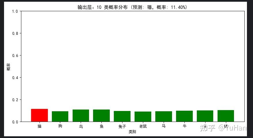
8. 输出层：分类结果

• 输入：84 维向量
• 输出：10 个神经元（10 分类）
• 原始 LeNet-5 使用 欧式径向基函数（RBF） ，现代版本几乎都替换为 全连接 + Softmax，将输出转为概率。

数据变换 ：84 维 → 10 维（各类别概率）

# 定义输出层（全连接 + Softmax）
output_layer = nn.Linear(in_features=84, out_features=10)
print(f"输出层参数量: {sum(p.numel() for p in output_layer.parameters())} 个")

class_names = ['猫', '狗', '鸟', '鱼', '兔子', '老鼠', '马', '牛', '羊', '猪']

with torch.no_grad():
    logits = output_layer(f6_output)
    probabilities = F.softmax(logits, dim=0)

print(f"\n输出 logits (未归一化):")
for i, (name, logit) in enumerate(zip(class_names, logits)):
    print(f"  {name}: {logit:.4f}")

print(f"\n输出概率 (Softmax 归一化后，和为 {probabilities.sum():.4f}):")
for i, (name, prob) in enumerate(zip(class_names, probabilities)):
    bar = '█' * int(prob * 50)
    print(f"  {name}: {prob:.4f} {bar}")

# 可视化概率分布
plt.figure(figsize=(10, 5))
bars = plt.bar(class_names, probabilities.numpy(), color='green')
pred_idx = probabilities.argmax().item()
bars[pred_idx].set_color('red')
plt.title(f'输出层：10 类概率分布 (预测: {class_names[pred_idx]}，概率: {probabilities[pred_idx]:.2%})')
plt.xlabel('类别')
plt.ylabel('概率')
plt.ylim(0, 1)
plt.show()
输出层参数量: 850 个

输出 logits (未归一化):
  猫: 0.1161
  狗: -0.0900
  鸟: 0.0590
  鱼: 0.0530
  兔子: -0.0602
  老鼠: -0.1348
  马: -0.0980
  牛: -0.0384
  羊: -0.0054
  猪: 0.0171

输出概率 (Softmax 归一化后，和为 1.0000):
  猫: 0.1140 █████
  狗: 0.0928 ████
  鸟: 0.1077 █████
  鱼: 0.1071 █████
  兔子: 0.0956 ████
  老鼠: 0.0887 ████
  马: 0.0921 ████
  牛: 0.0977 ████
  羊: 0.1010 █████
  猪: 0.1033 █████

输出层：10 类概率分布:

9. 完整 LeNet-5 模型定义与汇总

下面将所有层组合成一个完整的 LeNet-5 模型，并统计参数量。

class LeNet5(nn.Module):
    def __init__(self, num_classes=10):
        super(LeNet5, self).__init__()
        # 卷积层部分
        self.conv1 = nn.Conv2d(1, 6, kernel_size=5)   # C1
        self.pool1 = nn.AvgPool2d(2, stride=2)        # S2
        self.conv2 = nn.Conv2d(6, 16, kernel_size=5)  # C3
        self.pool2 = nn.AvgPool2d(2, stride=2)        # S4
        # 全连接层部分
        self.fc1 = nn.Linear(16 * 5 * 5, 120)         # C5 (以全连接方式实现)
        self.fc2 = nn.Linear(120, 84)                  # F6
        self.fc3 = nn.Linear(84, num_classes)          # 输出层
    
    def forward(self, x):
        x = torch.tanh(self.conv1(x))    # C1 + tanh
        x = self.pool1(x)                # S2 平均池化
        x = torch.tanh(self.conv2(x))    # C3 + tanh
        x = self.pool2(x)                # S4 平均池化
        x = x.view(x.size(0), -1)        # 展平
        x = torch.tanh(self.fc1(x))      # C5 + tanh
        x = torch.tanh(self.fc2(x))      # F6 + tanh
        x = self.fc3(x)                  # 输出层 (logits)
        return x

# 实例化模型
model = LeNet5(num_classes=10)
print(model)

# 统计总参数量
total_params = sum(p.numel() for p in model.parameters())
trainable_params = sum(p.numel() for p in model.parameters() if p.requires_grad)
print(f"\n总参数量: {total_params:,} 个")
print(f"可训练参数量: {trainable_params:,} 个")

# 各层参数量统计
print("\n各层参数量统计:")
for name, param in model.named_parameters():
    print(f"  {name}: {param.numel():,} (shape: {list(param.shape)})")
LeNet5(
  (conv1): Conv2d(1, 6, kernel_size=(5, 5), stride=(1, 1))
  (pool1): AvgPool2d(kernel_size=2, stride=2, padding=0)
  (conv2): Conv2d(6, 16, kernel_size=(5, 5), stride=(1, 1))
  (pool2): AvgPool2d(kernel_size=2, stride=2, padding=0)
  (fc1): Linear(in_features=400, out_features=120, bias=True)
  (fc2): Linear(in_features=120, out_features=84, bias=True)
  (fc3): Linear(in_features=84, out_features=10, bias=True)
)

总参数量: 61,706 个
可训练参数量: 61,706 个

各层参数量统计:
  conv1.weight: 150 (shape: [6, 1, 5, 5])
  conv1.bias: 6 (shape: [6])
  conv2.weight: 2,400 (shape: [16, 6, 5, 5])
  conv2.bias: 16 (shape: [16])
  fc1.weight: 48,000 (shape: [120, 400])
  fc1.bias: 120 (shape: [120])
  fc2.weight: 10,080 (shape: [84, 120])
  fc2.bias: 84 (shape: [84])
  fc3.weight: 840 (shape: [10, 84])
  fc3.bias: 10 (shape: [10])
# 用完整模型做一次前向传播，验证与之前逐层计算结果一致
with torch.no_grad():
    final_output = model(input_tensor)
    final_prob = F.softmax(final_output, dim=1)

print(f"模型输入: {input_tensor.shape}")
print(f"模型输出: {final_output.shape}")
print(f"预测类别: {class_names[final_prob.argmax().item()]} (概率: {final_prob.max():.2%})")

# 验证：用完整模型的权重和手动逐层计算的结果对比
# （注意：因为权重初始化是随机的，这里只验证维度是否正确）
print("\n=== 完整数据流尺寸变换 ===")
x = input_tensor
print(f"输入: {list(x.shape)}")
x = torch.tanh(model.conv1(x))
print(f"C1 (Conv2d + tanh): {list(x.shape)}")
x = model.pool1(x)
print(f"S2 (AvgPool2d): {list(x.shape)}")
x = torch.tanh(model.conv2(x))
print(f"C3 (Conv2d + tanh): {list(x.shape)}")
x = model.pool2(x)
print(f"S4 (AvgPool2d): {list(x.shape)}")
x = x.view(x.size(0), -1)
print(f"Flatten: {list(x.shape)}")
x = torch.tanh(model.fc1(x))
print(f"C5 (Linear + tanh): {list(x.shape)}")
x = torch.tanh(model.fc2(x))
print(f"F6 (Linear + tanh): {list(x.shape)}")
x = model.fc3(x)
print(f"输出层 (Linear): {list(x.shape)}")
模型输入: torch.Size([1, 1, 32, 32])
模型输出: torch.Size([1, 10])
预测类别: 狗 (概率: 11.71%)

=== 完整数据流尺寸变换 ===
输入: [1, 1, 32, 32]
C1 (Conv2d + tanh): [1, 6, 28, 28]
S2 (AvgPool2d): [1, 6, 14, 14]
C3 (Conv2d + tanh): [1, 16, 10, 10]
S4 (AvgPool2d): [1, 16, 5, 5]
Flatten: [1, 400]
C5 (Linear + tanh): [1, 120]
F6 (Linear + tanh): [1, 84]
输出层 (Linear): [1, 10]

10. 用 MNIST 训练 LeNet-5（演示训练过程）

为了展示完整的训练过程，我们用经典的 MNIST 手写数字数据集来训练这个 LeNet-5 模型。猫咪图片只是用来演示数据流，真正的训练需要大规模标注数据。

import torch.optim as optim
from torchvision import datasets
from torch.utils.data import DataLoader

# MNIST 数据预处理
train_transform = transforms.Compose([
    transforms.Resize((32, 32)),  # LeNet-5 输入是 32×32
    transforms.ToTensor(),
])

# 加载 MNIST 数据集（如果没有会自动下载）
train_dataset = datasets.MNIST(
    root='./data', train=True, download=True, transform=train_transform
)
test_dataset = datasets.MNIST(
    root='./data', train=False, download=True, transform=train_transform
)

train_loader = DataLoader(train_dataset, batch_size=64, shuffle=True)
test_loader = DataLoader(test_dataset, batch_size=1000, shuffle=False)

print(f"训练集大小: {len(train_dataset)} 张")
print(f"测试集大小: {len(test_dataset)} 张")
print(f"批次大小: 64")

# 显示一些训练样本
images, labels = next(iter(train_loader))
fig, axes = plt.subplots(2, 8, figsize=(12, 3))
for i in range(16):
    ax = axes[i // 8, i % 8]
    ax.imshow(images[i, 0], cmap='gray')
    ax.set_title(f'标签: {labels[i].item()}')
    ax.axis('off')
plt.suptitle('MNIST 训练样本示例')
plt.tight_layout()
plt.show()
# 训练配置
device = torch.device('cuda' if torch.cuda.is_available() else 'cpu')
print(f"训练设备: {device}")

model = LeNet5(num_classes=10).to(device)
criterion = nn.CrossEntropyLoss()
optimizer = optim.Adam(model.parameters(), lr=0.001)

epochs = 5
train_losses = []
train_accs = []
test_accs = []

for epoch in range(epochs):
    model.train()
    running_loss = 0.0
    correct = 0
    total = 0
    
    for batch_idx, (images, labels) in enumerate(train_loader):
        images, labels = images.to(device), labels.to(device)
        
        optimizer.zero_grad()
        outputs = model(images)
        loss = criterion(outputs, labels)
        loss.backward()
        optimizer.step()
        
        running_loss += loss.item()
        _, predicted = outputs.max(1)
        total += labels.size(0)
        correct += predicted.eq(labels).sum().item()
    
    train_loss = running_loss / len(train_loader)
    train_acc = 100. * correct / total
    train_losses.append(train_loss)
    train_accs.append(train_acc)
    
    # 测试集评估
    model.eval()
    test_correct = 0
    test_total = 0
    with torch.no_grad():
        for images, labels in test_loader:
            images, labels = images.to(device), labels.to(device)
            outputs = model(images)
            _, predicted = outputs.max(1)
            test_total += labels.size(0)
            test_correct += predicted.eq(labels).sum().item()
    
    test_acc = 100. * test_correct / test_total
    test_accs.append(test_acc)
    
    print(f"Epoch [{epoch+1}/{epochs}] "
          f"训练损失: {train_loss:.4f}, "
          f"训练准确率: {train_acc:.2f}%, "
          f"测试准确率: {test_acc:.2f}%")

print("\n训练完成！")
# 可视化训练过程
fig, axes = plt.subplots(1, 2, figsize=(14, 5))

# 损失曲线
axes[0].plot(range(1, epochs+1), train_losses, 'b-o', label='训练损失')
axes[0].set_title('训练损失曲线')
axes[0].set_xlabel('Epoch')
axes[0].set_ylabel('Loss')
axes[0].legend()
axes[0].grid(True, alpha=0.3)

# 准确率曲线
axes[1].plot(range(1, epochs+1), train_accs, 'r-o', label='训练准确率')
axes[1].plot(range(1, epochs+1), test_accs, 'g-s', label='测试准确率')
axes[1].set_title('准确率变化')
axes[1].set_xlabel('Epoch')
axes[1].set_ylabel('准确率 (%)')
axes[1].legend()
axes[1].grid(True, alpha=0.3)

plt.tight_layout()
plt.show()

print(f"最终测试准确率: {test_accs[-1]:.2f}%")

11. 总结：一张图看懂 LeNet-5 的数据流

层名称	类型	输入尺寸	输出尺寸	核心参数 / 说明
输入	灰度图	32×32×1	32×32×1	猫咪照片 / MNIST 数字
C1	卷积 + tanh	32×32×1	28×28×6	6 个 5×5 核，156 个参数
S2	平均池化	28×28×6	14×14×6	2×2 窗口，步长 2
C3	卷积 + tanh	14×14×6	10×10×16	16 组 5×5 核，2416 参
S4	平均池化	10×10×16	5×5×16	2×2 窗口，步长 2
C5	全连接 + tanh	5×5×16=400	120	48120 个参数
F6	全连接 + tanh	120	84	10164 个参数
输出	全连接 + Softmax	84	10	850 个参数，输出各类概率

从猫咪图片的原始像素开始，网络先用卷积提取边缘和纹理，用池化压缩并固化特征，再用多层卷积组合出更高级特征，最后在全连接层进行抽象并输出分类结果。整个过程层层递进，完美诠释了卷积神经网络的层次化特征学习。

编辑于 2026-06-25 11:54・安徽・包含 AI 辅助创作 作者对内容负责

[

卷积神经网络（CNN）

](https://www.zhihu.com/topic/20043586)