数字图像处理：直方图应用

数字图像处理：直方图应用

在数字图像处理中，直方图是一种重要的图像分析工具。它描述了图像中像素灰度值的分布情况，是图像增强、分割、特征提取等许多图像处理技术的基础。本章将介绍直方图的几个重要应用，包括直方图均衡化、直方图匹配、局部直方图处理以及图像增强中的直方图统计方法。

# -*- coding: utf-8 -*-
# 数字图像处理：直方图应用
# 
# 本Notebook演示直方图在数字图像处理中的几个重要应用：
# 1. 直方图均衡化
# 2. 直方图匹配（规定化）
# 3. 均衡化与规定化对比
# 4. 局部直方图处理（CLAHE）
# 5. 图像增强中的直方图统计

# ============ 导入必要的库 ============
# cv2: OpenCV库，用于图像处理
# numpy: 数值计算库，用于数组操作
# matplotlib.pyplot: 绘图库，用于显示图像和直方图
import cv2
import numpy as np
import matplotlib.pyplot as plt

# ============ 设置中文显示 ============
# 设置matplotlib的中文字体，避免中文显示为方框
plt.rcParams['font.sans-serif'] = ['SimHei', 'Microsoft YaHei']
# 解决负号显示问题
plt.rcParams['axes.unicode_minus'] = False

# ============ 读取用户图片 ============
# 使用用户提供的图片，路径相对于Notebook所在目录
# cv2.IMREAD_GRAYSCALE: 以灰度模式读取图像
image_path = 'images/fX315vbEs.jpeg'
img = cv2.imread(image_path, cv2.IMREAD_GRAYSCALE)

# 检查图像是否成功读取
if img is None:
    raise ValueError(f"无法读取图像文件: {image_path}\n请确保图片文件存在且路径正确。")

# 打印图像基本信息
print(f"图像路径: {image_path}")
print(f"图像形状: {img.shape} (高度 x 宽度)")
print(f"灰度范围: [{img.min()}, {img.max()}]")
print(f"像素总数: {img.size}")
图像路径: images/fX315vbEs.jpeg
图像形状: (263, 647) (高度 x 宽度)
灰度范围: [0, 255]
像素总数: 170161

1.1 直方图均衡

直方图均衡化是一种经典的图像增强技术，其目的是通过拉伸图像的直方图，使灰度值均匀分布在整个动态范围内。核心思想是将原始图像的累积分布函数转换为均匀分布的CDF。

为什么要进行直方图均衡化

• 增强对比度：对于对比度较低的图像，直方图均衡化可以显著提高视觉效果

• 扩展动态范围：将集中在较窄范围内的灰度值扩展到整个动态范围

• 改善视觉质量：使图像更加清晰，细节更加明显

优点

• 操作简单，计算效率高

• 不需要先验知识

• 自动适应图像的灰度分布

• 对多种类型的图像都有效

# ============ 1.1.4 直方图均衡化代码实现 ============
# 
# 使用第一个代码cell中已经读取的图片 img
# 如果需要使用其他图片，可以修改 image_path 变量

# ------------------
# 函数1: 计算直方图
# ------------------
# 输入: 灰度图像 img (numpy数组)
# 输出: 直方图 hist (长度为256的数组，hist[i]表示灰度值为i的像素数)
# 
# 原理: 遍历图像中每个像素，统计每个灰度值出现的次数
def compute_histogram(img):
    # 创建长度为256的数组，初始化为0，用于存储每个灰度值的像素数
    hist = np.zeros(256, dtype=np.int32)
    
    # 获取图像的高度和宽度
    height, width = img.shape
    
    # 遍历图像的每个像素
    for i in range(height):
        for j in range(width):
            # 获取当前像素的灰度值
            gray_value = img[i, j]
            # 对应灰度值的计数加1
            hist[gray_value] += 1
    
    return hist

# ------------------
# 函数2: 直方图均衡化
# ------------------
# 输入: 灰度图像 img (numpy数组)
# 输出: 
#   equalized_img: 均衡化后的图像
#   cdf_normalized: 归一化的累积分布函数
# 
# 原理: 
# 1. 计算原始图像的直方图
# 2. 计算累积分布函数(CDF)
# 3. 将CDF归一化到[0, 255]范围
# 4. 使用归一化的CDF作为查找表，将原始图像映射到均衡化后的图像
# 
# 数学公式: s = T(r) = (L-1) * integral(0 to r) p_r(w) dw
# 其中 L=256, p_r(r)是原始图像的概率密度函数
def histogram_equalization(img):
    # 步骤1: 计算原始图像的直方图
    hist = compute_histogram(img)
    
    # 步骤2: 计算累积分布函数(CDF)
    # CDF[i] = sum_{k=0}^{i} hist[k]
    cdf = hist.cumsum()
    
    # 步骤3: 将CDF归一化到[0, 255]范围
    # cdf[-1]是CDF的最后一个值，即图像的总像素数
    cdf_normalized = cdf * 255 / cdf[-1]
    
    # 步骤4: 使用归一化的CDF作为查找表，映射原始图像
    # cdf_normalized[img] 将每个像素的灰度值替换为对应的CDF值
    equalized_img = cdf_normalized[img].astype(np.uint8)
    
    return equalized_img, cdf_normalized

# ============ 执行直方图均衡化 ============
# 使用第一个cell中读取的图片进行均衡化
equalized_img, cdf = histogram_equalization(img)

# ============ 计算原图和均衡化后图像的直方图 ============
hist_original = compute_histogram(img)
hist_equalized = compute_histogram(equalized_img)

# ============ 绘制对比图 ============
# 创建2行2列的子图，图大小为12x10
fig, axes = plt.subplots(2, 2, figsize=(12, 10))

# 子图1: 原图
axes[0, 0].imshow(img, cmap='gray')
axes[0, 0].set_title('1. 原图')
axes[0, 0].axis('off')  # 关闭坐标轴

# 子图2: 原图直方图
axes[0, 1].bar(range(256), hist_original, width=1.0, color='gray')
axes[0, 1].set_title('2. 原图直方图')
axes[0, 1].set_xlabel('灰度值')
axes[0, 1].set_ylabel('像素数')
axes[0, 1].set_xlim([0, 255])  # 设置x轴范围

# 子图3: 均衡化后图像
axes[1, 0].imshow(equalized_img, cmap='gray')
axes[1, 0].set_title('3. 直方图均衡化后')
axes[1, 0].axis('off')

# 子图4: 均衡化后直方图
axes[1, 1].bar(range(256), hist_equalized, width=1.0, color='gray')
axes[1, 1].set_title('4. 均衡化后直方图')
axes[1, 1].set_xlabel('灰度值')
axes[1, 1].set_ylabel('像素数')
axes[1, 1].set_xlim([0, 255])

# 调整子图间距
plt.tight_layout()

# 显示图像
plt.show()

# ============ 输出统计信息 ============
print("=== 直方图均衡化统计 ===")
print(f"原图灰度范围: [{img.min()}, {img.max()}]")
print(f"均衡化后灰度范围: [{equalized_img.min()}, {equalized_img.max()}]")
print(f"原图均值: {img.mean():.2f}")
print(f"均衡化后均值: {equalized_img.mean():.2f}")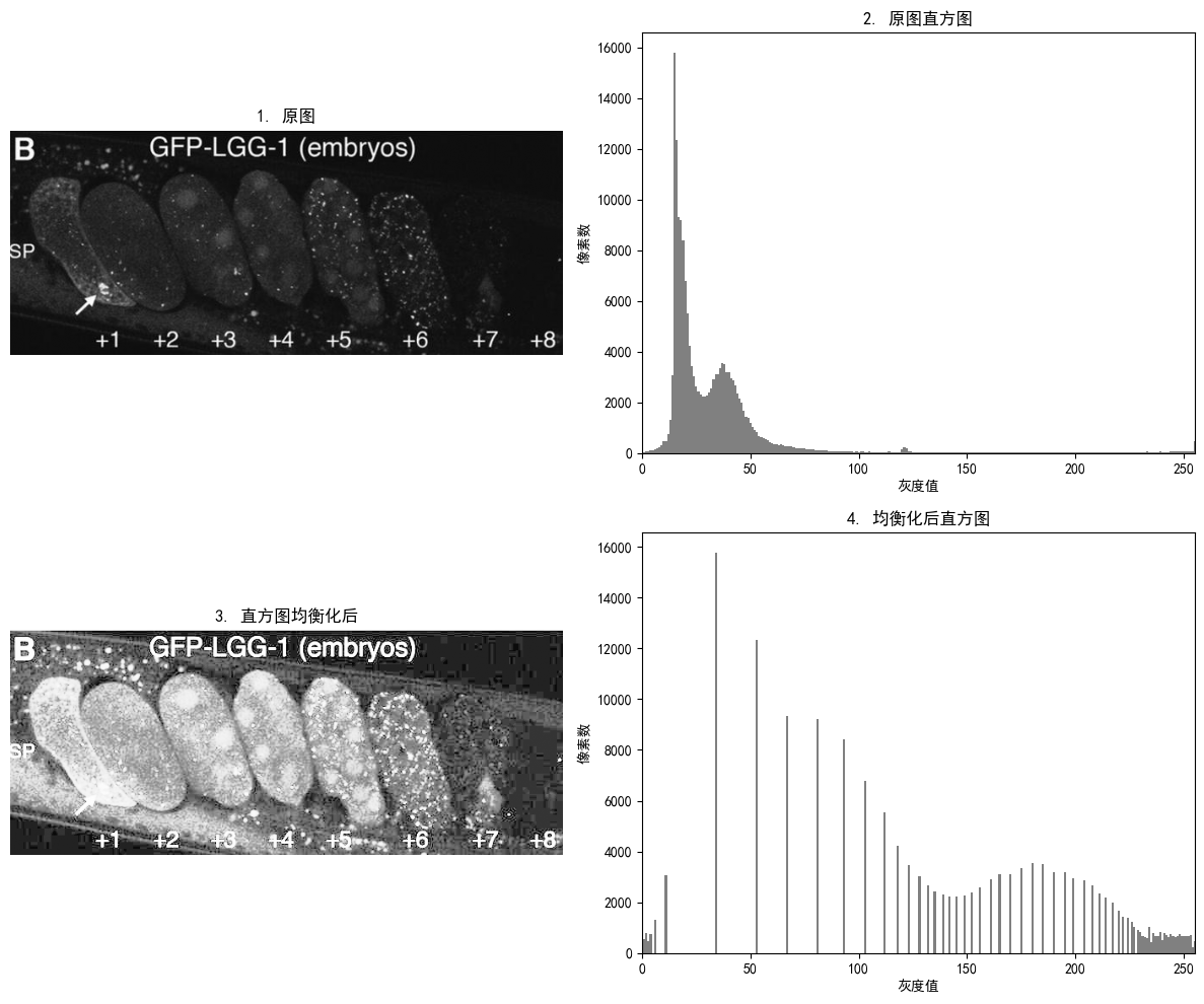

添加图片注释，不超过 140 字（可选）

=== 直方图均衡化统计 ===
原图灰度范围: [0, 255]
均衡化后灰度范围: [0, 255]
原图均值: 34.44
均衡化后均值: 131.19

从上述对比图可以看出：原图是低对比度图像，灰度值集中在较窄范围内；均衡化后对比度明显增强，灰度值分布更加均匀。直方图均衡化成功地将集中的灰度值扩展到了整个动态范围。

1.2 直方图匹配（规定化）

直方图匹配是一种将图像的直方图调整为指定目标直方图的技术。与直方图均衡化不同，直方图匹配可以根据需求灵活地控制图像的灰度分布。

为什么要进行直方图匹配

• 灵活控制：可以根据需要将图像调整为任意目标直方图

• 风格统一：在多图像处理中，可以使不同图像具有相同的灰度分布风格

• 特定增强：针对特定应用场景，可以定制直方图

优点

• 比直方图均衡化更灵活

• 可以实现特定的视觉效果

• 适用于需要统一风格的图像处理任务

def create_target_histogram(type='uniform'):
    if type == 'uniform':
        return np.ones(256, dtype=np.int32) * 100
    elif type == 'gaussian':
        x = np.arange(256)
        mean = 128
        std = 40
        return np.int32(np.exp(-(x - mean)**2 / (2 * std**2)) * 5000)
    elif type == 'bimodal':
        x = np.arange(256)
        h1 = np.exp(-(x - 64)**2 / (2 * 20**2)) * 3000
        h2 = np.exp(-(x - 192)**2 / (2 * 20**2)) * 3000
        return np.int32(h1 + h2)

def match_to_target_histogram(img, target_hist):
    src_hist = compute_histogram(img)
    src_cdf = src_hist.cumsum()
    src_cdf_normalized = src_cdf * 255 / src_cdf[-1]
    
    target_cdf = target_hist.cumsum()
    target_cdf_normalized = target_cdf * 255 / target_cdf[-1]
    
    mapping = np.zeros(256, dtype=np.uint8)
    j = 0
    for i in range(256):
        while j < 255 and target_cdf_normalized[j] < src_cdf_normalized[i]:
            j += 1
        mapping[i] = j
    
    return mapping[img]

# 使用第一个cell中读取的用户图片
src_img = img

target_hist_uniform = create_target_histogram('uniform')
target_hist_gaussian = create_target_histogram('gaussian')
target_hist_bimodal = create_target_histogram('bimodal')

matched_uniform = match_to_target_histogram(src_img, target_hist_uniform)
matched_gaussian = match_to_target_histogram(src_img, target_hist_gaussian)
matched_bimodal = match_to_target_histogram(src_img, target_hist_bimodal)

hist_src = compute_histogram(src_img)
hist_uniform = compute_histogram(matched_uniform)
hist_gaussian = compute_histogram(matched_gaussian)
hist_bimodal = compute_histogram(matched_bimodal)

fig, axes = plt.subplots(2, 4, figsize=(20, 10))

axes[0, 0].imshow(src_img, cmap='gray')
axes[0, 0].set_title('1. 原图')
axes[0, 0].axis('off')

axes[1, 0].bar(range(256), hist_src, width=1.0, color='gray')
axes[1, 0].set_title('原图直方图')
axes[1, 0].set_xlim([0, 255])
axes[1, 0].set_xticks([])

axes[0, 1].imshow(matched_uniform, cmap='gray')
axes[0, 1].set_title('2. 均匀分布匹配')
axes[0, 1].axis('off')

axes[1, 1].bar(range(256), hist_uniform, width=1.0, color='gray')
axes[1, 1].set_title('均匀分布直方图')
axes[1, 1].set_xlim([0, 255])
axes[1, 1].set_xticks([])

axes[0, 2].imshow(matched_gaussian, cmap='gray')
axes[0, 2].set_title('3. 高斯分布匹配')
axes[0, 2].axis('off')

axes[1, 2].bar(range(256), hist_gaussian, width=1.0, color='gray')
axes[1, 2].set_title('高斯分布直方图')
axes[1, 2].set_xlim([0, 255])
axes[1, 2].set_xticks([])

axes[0, 3].imshow(matched_bimodal, cmap='gray')
axes[0, 3].set_title('4. 双峰分布匹配')
axes[0, 3].axis('off')

axes[1, 3].bar(range(256), hist_bimodal, width=1.0, color='gray')
axes[1, 3].set_title('双峰分布直方图')
axes[1, 3].set_xlim([0, 255])
axes[1, 3].set_xticks([])

plt.tight_layout()
plt.show()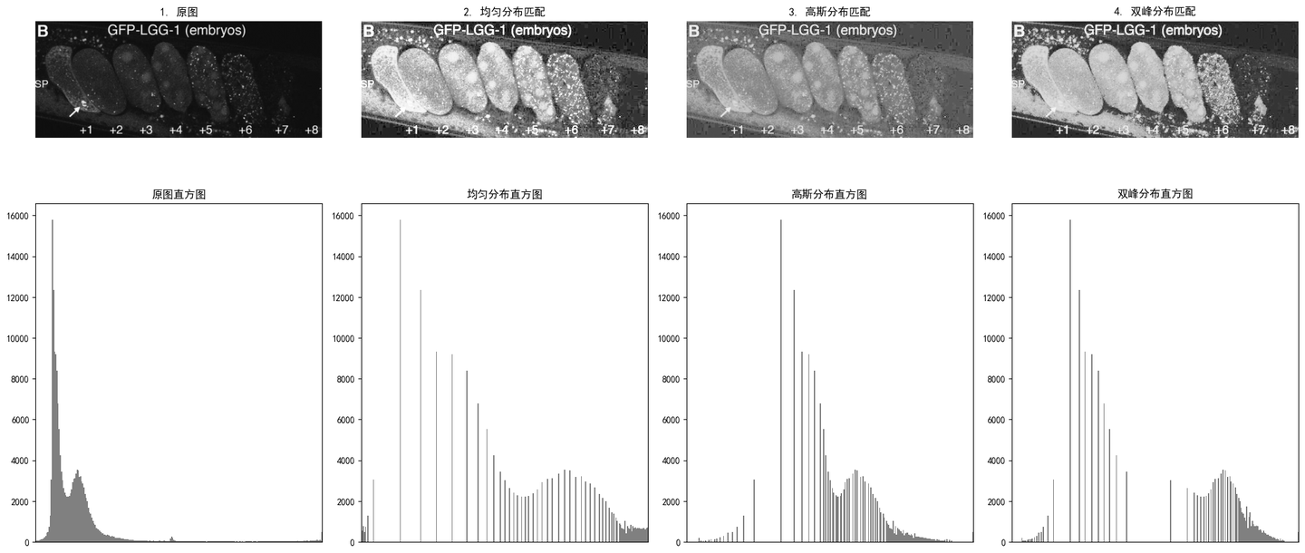

添加图片注释，不超过 140 字（可选）

从上述对比图可以看出：均匀分布匹配类似于直方图均衡化；高斯分布匹配使图像灰度值集中在中间区域，产生柔和效果；双峰分布匹配使图像呈现明显的亮暗分区效果。直方图匹配提供了灵活的方式来控制图像的灰度分布。

1.3 均衡和规定化对比

原理对比

# 使用第一个cell中读取的用户图片\n

equalized_img, _ = histogram_equalization(img)
matched_img = match_to_target_histogram(img, create_target_histogram('uniform'))

hist_original = compute_histogram(img)
hist_equalized = compute_histogram(equalized_img)
hist_matched = compute_histogram(matched_img)

fig, axes = plt.subplots(3, 2, figsize=(14, 16))

axes[0, 0].imshow(img, cmap='gray')
axes[0, 0].set_title('1. 原图')
axes[0, 0].axis('off')

axes[0, 1].bar(range(256), hist_original, width=1.0, color='gray')
axes[0, 1].set_title('原图直方图')
axes[0, 1].set_xlim([0, 255])

axes[1, 0].imshow(equalized_img, cmap='gray')
axes[1, 0].set_title('2. 直方图均衡化')
axes[1, 0].axis('off')

axes[1, 1].bar(range(256), hist_equalized, width=1.0, color='gray')
axes[1, 1].set_title('均衡化后直方图')
axes[1, 1].set_xlim([0, 255])

axes[2, 0].imshow(matched_img, cmap='gray')
axes[2, 0].set_title('3. 直方图规定化（均匀目标）')
axes[2, 0].axis('off')

axes[2, 1].bar(range(256), hist_matched, width=1.0, color='gray')
axes[2, 1].set_title('规定化后直方图')
axes[2, 1].set_xlim([0, 255])

plt.tight_layout()
plt.show()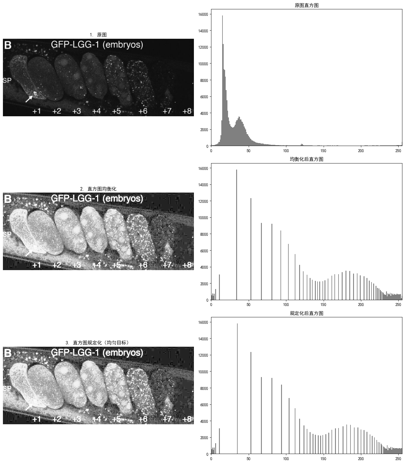

添加图片注释，不超过 140 字（可选）

对比分析

直方图均衡化自动将直方图均匀化，对比度增强效果明显，但无法控制最终的直方图形状；直方图规定化需要指定目标直方图，可以精确控制图像的灰度分布。当目标为均匀分布时，效果与均衡化类似，但可能略有差异。

适用场景总结

• 直方图均衡化：适用于需要快速增强图像对比度，且对最终直方图形状没有特定要求的场景

• 直方图规定化：适用于需要将图像调整为特定风格，或需要统一多幅图像灰度分布的场景

1.4 局部直方图处理

全局直方图处理是对整个图像进行统一处理，这在光照不均匀的图像中可能会导致部分区域过度增强或增强不足。局部直方图处理则是对图像的每个局部区域单独进行直方图调整。

为什么要进行局部直方图处理

• 处理光照不均匀：全局处理无法有效处理光照变化较大的图像

• 保留局部细节：不同区域可能需要不同程度的增强

• 避免过度增强：防止局部区域对比度过度增强导致失真

优点

• 能够有效处理光照不均匀的图像

• 保留图像的局部细节

• 避免全局处理可能导致的问题

# 使用第一个cell中读取的用户图片\n
# img = image_uneven  # 已注释，使用用户图片\n

# ============ 全局直方图均衡化 ============
# 使用之前定义的直方图均衡化函数对整幅图像进行处理
# 全局均衡化可能会导致局部区域过度增强或增强不足
global_equalized, _ = histogram_equalization(img)

# ============ CLAHE（对比度受限的自适应直方图均衡化） ============
# CLAHE是一种局部直方图处理技术，通过以下方式改进传统的自适应直方图均衡化：
# 1. 将图像分成多个小区域（tiles）
# 2. 对每个tile单独进行直方图均衡化
# 3. 使用限制对比度（clipLimit）来防止噪声放大
# 
# 参数说明：
# - clipLimit: 对比度限制阈值，默认40.0。当某个灰度级的像素数超过此阈值时，
#   超出部分会被均匀分配到其他灰度级，防止过度增强导致噪声放大
# - tileGridSize: 图像分割的网格大小，(8, 8)表示将图像分成8x8=64个小区域
#   每个区域独立进行直方图均衡化
clahe = cv2.createCLAHE(clipLimit=2.0, tileGridSize=(8, 8))

# 对图像应用CLAHE处理
clahe_img = clahe.apply(img)

hist_original = compute_histogram(img)
hist_global = compute_histogram(global_equalized)
hist_clahe = compute_histogram(clahe_img)

fig, axes = plt.subplots(3, 2, figsize=(14, 16))

axes[0, 0].imshow(img, cmap='gray')
axes[0, 0].set_title('1. 原图（光照不均匀）')
axes[0, 0].axis('off')

axes[0, 1].bar(range(256), hist_original, width=1.0, color='gray')
axes[0, 1].set_title('原图直方图')
axes[0, 1].set_xlim([0, 255])

axes[1, 0].imshow(global_equalized, cmap='gray')
axes[1, 0].set_title('2. 全局直方图均衡化')
axes[1, 0].axis('off')

axes[1, 1].bar(range(256), hist_global, width=1.0, color='gray')
axes[1, 1].set_title('全局均衡化后直方图')
axes[1, 1].set_xlim([0, 255])

axes[2, 0].imshow(clahe_img, cmap='gray')
axes[2, 0].set_title('3. CLAHE局部直方图均衡化')
axes[2, 0].axis('off')

axes[2, 1].bar(range(256), hist_clahe, width=1.0, color='gray')
axes[2, 1].set_title('CLAHE后直方图')
axes[2, 1].set_xlim([0, 255])

plt.tight_layout()
plt.show()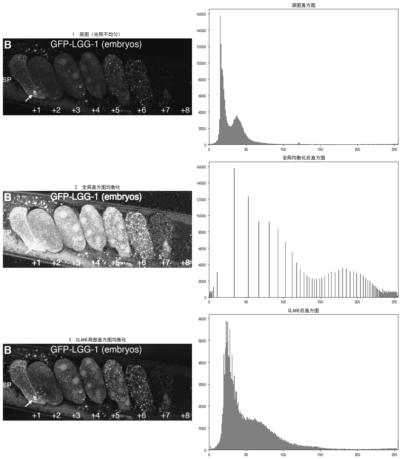

添加图片注释，不超过 140 字（可选）

从上述对比图可以看出：原图存在明显的光照不均匀；全局直方图均衡化虽然增强了整体对比度，但暗区域和亮区域的处理效果不一致；CLAHE局部直方图均衡化有效地处理了光照不均匀问题，各个区域的对比度都得到了适当增强。

1.5 图像增强中直方图统计

直方图统计是利用直方图的统计特性来进行图像增强的方法。常用统计量包括均值、方差、最小值、最大值等。

基于直方图统计的增强方法

方法一：直方图拉伸

方法二：直方图截断

方法三：阈值处理

def compute_histogram_stats(img):
    hist = compute_histogram(img)
    mean = np.sum(np.arange(256) * hist) / np.sum(hist)
    variance = np.sum((np.arange(256) - mean)**2 * hist) / np.sum(hist)
    min_val = np.min(img)
    max_val = np.max(img)
    dynamic_range = max_val - min_val
    return {
        'mean': mean,
        'variance': variance,
        'std': np.sqrt(variance),
        'min': min_val,
        'max': max_val,
        'dynamic_range': dynamic_range
    }

def contrast_stretching(img):
    min_val = np.min(img)
    max_val = np.max(img)
    if max_val == min_val:
        return img
    stretched_img = ((img - min_val) / (max_val - min_val) * 255).astype(np.uint8)
    return stretched_img

def histogram_clipping(img, lower_percent=5, upper_percent=95):
    lower_val = np.percentile(img, lower_percent)
    upper_val = np.percentile(img, upper_percent)
    clipped_img = np.clip(img, lower_val, upper_val)
    clipped_img = ((clipped_img - lower_val) / (upper_val - lower_val) * 255).astype(np.uint8)
    return clipped_img

def thresholding(img, threshold=None):
    if threshold is None:
        _, threshold = cv2.threshold(img, 0, 255, cv2.THRESH_BINARY + cv2.THRESH_OTSU)
    binary_img = (img >= threshold).astype(np.uint8) * 255
    return binary_img, threshold

# 使用第一个cell中读取的用户图片\n
# img = image_low_contrast  # 已注释，使用用户图片\n

stats = compute_histogram_stats(img)
print("图像统计信息:")
print(f"  均值: {stats['mean']:.2f}")
print(f"  标准差: {stats['std']:.2f}")
print(f"  最小值: {stats['min']}")
print(f"  最大值: {stats['max']}")
print(f"  动态范围: {stats['dynamic_range']}")

stretched_img = contrast_stretching(img)
clipped_img = histogram_clipping(img)
binary_img, otsu_threshold = thresholding(img)

hist_original = compute_histogram(img)
hist_stretched = compute_histogram(stretched_img)
hist_clipped = compute_histogram(clipped_img)
hist_binary = compute_histogram(binary_img)

fig, axes = plt.subplots(4, 2, figsize=(14, 20))

axes[0, 0].imshow(img, cmap='gray')
axes[0, 0].set_title(f'1. 原图 (均值={stats["mean"]:.1f}, 动态范围={stats["dynamic_range"]})')
axes[0, 0].axis('off')

axes[0, 1].bar(range(256), hist_original, width=1.0, color='gray')
axes[0, 1].set_title('原图直方图')
axes[0, 1].set_xlim([0, 255])

axes[1, 0].imshow(stretched_img, cmap='gray')
axes[1, 0].set_title('2. 直方图拉伸')
axes[1, 0].axis('off')

axes[1, 1].bar(range(256), hist_stretched, width=1.0, color='gray')
axes[1, 1].set_title('拉伸后直方图')
axes[1, 1].set_xlim([0, 255])

axes[2, 0].imshow(clipped_img, cmap='gray')
axes[2, 0].set_title('3. 直方图截断（5%-95%）')
axes[2, 0].axis('off')

axes[2, 1].bar(range(256), hist_clipped, width=1.0, color='gray')
axes[2, 1].set_title('截断后直方图')
axes[2, 1].set_xlim([0, 255])

axes[3, 0].imshow(binary_img, cmap='gray')
axes[3, 0].set_title(f'4. 阈值处理（Otsu阈值={otsu_threshold}）')
axes[3, 0].axis('off')

axes[3, 1].bar(range(256), hist_binary, width=1.0, color='gray')
axes[3, 1].set_title('二值化后直方图')
axes[3, 1].set_xlim([0, 255])

plt.tight_layout()
plt.show()
图像统计信息:
  均值: 34.44
  标准差: 33.71
  最小值: 0
  最大值: 255
  动态范围: 255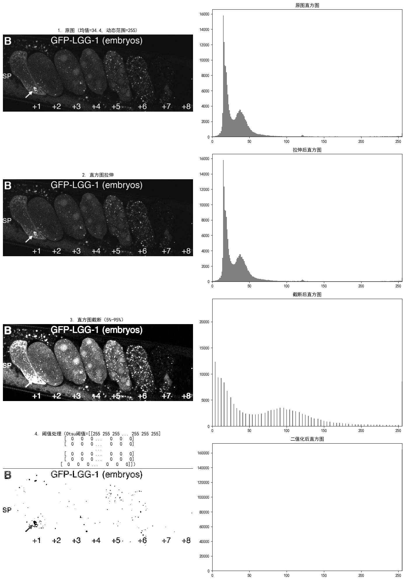

添加图片注释，不超过 140 字（可选）

从上述对比图可以看出：直方图拉伸将灰度范围扩展到整个动态范围；直方图截断去除了极端值的影响，增强效果更加自然；阈值处理使用Otsu方法自动确定阈值，将图像转换为二值图像。

方法选择建议

• 直方图拉伸：适用于灰度范围较小的图像，简单有效

• 直方图截断：适用于存在极端值噪声的图像

• 阈值处理：适用于需要二值化的场景

总结

1. 直方图均衡化：通过均匀化直方图来增强图像对比度

2. 直方图匹配（规定化）：将图像直方图调整为指定目标直方图

3. 均衡化与规定化对比：均衡化简单通用，规定化灵活可控

4. 局部直方图处理：针对光照不均匀的图像，使用局部区域处理

5. 图像增强中直方图统计：利用直方图的统计特性进行定量分析

这些方法在实际应用中各有侧重，选择合适的方法取决于具体的图像特征和应用需求。