Since many students in my Stat 451: Introduction to Machine Learning and Statistical Pattern Classification class are relatively new to Python and NumPy, I was recently devoting a lecture to the latter. Since the course notes are based on an interactive Jupyter notebook file, which I used as a basis for the lecture videos, I thought it would be worthwhile to reformat it as a blog article with the embedded "narrated content" -- the video recordings.
由于我的Stat 451:机器学习和统计模式分类导论课上的许多学生对Python和NumPy相对较新,我最近专门为后者做了一场讲座。由于课程笔记基于一个交互式Jupyter笔记本文件,我将其用作讲座视频的基础,我认为将其重新格式化为一篇带有嵌入式"叙述内容"的博客文章是值得的------视频记录。
Additional Material:附加材料:
- Here is a link to a Deepnote version of this article that you can interact with in your browser.这是本文Deepnote版本的链接,您可以在浏览器中与之交互。
- A link to the Jupyter notebook version of this article can be found on GitHub at: https://github.com/rasbt/numpy-intro-blogarticle-2020.本文Jupyter笔记本版本的链接可以在GitHub上找到:https://github.com/rasbt/numpy-intro-blogarticle-2020 .
The code for this article was generated using the following software versions:
本文的代码是使用以下软件版本生成的:
- CPython 3.8.3
- numpy 1.19.1编号1.19.1
- matplotlib 3.3.1
4.1: NumPy Basics
NumPy -- Working with Numerical Arrays
Introduction to NumPy
This section offers a quick tour of the NumPy library for working with multi-dimensional arrays in Python. NumPy (short for Numerical Python) was created in 2005 by merging Numarray into Numeric. Since then, the open source NumPy library has evolved into an essential library for scientific computing in Python. It has become a building block of many other scientific libraries, such as SciPy, Scikit-learn, Pandas, and others.
What makes NumPy so incredibly attractive to the scientific community is that it provides a convenient Python interface for working with multi-dimensional array data structures efficiently; the NumPy array data structure is also called ndarray, which is short for n-dimensional array.
本节简要介绍了在Python中使用多维数组的NumPy库。NumPy(Numerical Python的缩写)于2005年通过将Numarray合并到Numeric中而创建。从那时起,开源NumPy库已经发展成为Python中科学计算的重要库。它已成为许多其他科学图书馆的组成部分,如SciPy、Scikit-learn、Pandas等。NumPy之所以对科学界极具吸引力,是因为它提供了一个方便的Python接口,可以高效地处理多维数组数据结构;NumPy数组数据结构也称为ndarray,是n维数组的缩写。
In addition to being mostly implemented in C and using Python as a "glue language," the main reason why NumPy is so efficient for numerical computations is that NumPy arrays use contiguous blocks of memory that can be efficiently cached by the CPU. In contrast, Python lists are arrays of pointers to objects in random locations in memory, which cannot be easily cached and come with a more expensive memory-look-up. However, the computational efficiency and low-memory footprint come at a cost: NumPy arrays have a fixed size and are homogeneous, which means that all elements must have the same type. Homogenous ndarray objects have the advantage that NumPy can carry out operations using efficient C code and avoid expensive type checks and other overheads of the Python API. While adding and removing elements from the end of a Python list is very efficient, altering the size of a NumPy array is very expensive since it requires to create a new array and carry over the contents of the old array that we want to expand or shrink.
除了主要用C实现并使用Python作为"粘合语言"外,NumPy在数值计算方面如此高效的主要原因是NumPy数组使用连续的内存块,CPU可以有效地缓存这些内存块。相比之下,Python列表是指向内存中随机位置的对象的指针数组,不容易缓存,并且需要更昂贵的内存查找。然而,计算效率和低内存占用是有代价的:NumPy数组具有固定大小并且是同构的,这意味着所有元素必须具有相同的类型。同源ndarray对象的优点是NumPy可以使用高效的C代码执行操作,并避免昂贵的类型检查和Python API的其他开销。虽然在Python列表末尾添加和删除元素非常有效,但更改NumPy数组的大小非常昂贵,因为它需要创建一个新数组并继承我们想要扩展或收缩的旧数组的内容。
Besides being more efficient for numerical computations than native Python code, NumPy can also be more elegant and readable due to vectorized operations and broadcasting, which are features that we will explore in this article.
除了比原生Python代码更高效地进行数值计算外,NumPy还可以通过矢量化操作和广播更优雅、更易读,这是我们将在本文中探讨的功能。
Today, NumPy forms the basis of the scientific Python computing ecosystem.
如今,NumPy构成了科学Python计算生态系统的基础。
Motivation: NumPy is fast!
Here is some motivation before we discuss further details, highlighting why learning about and using NumPy is useful. We take a look at a speed comparison with regular Python code. In particular, we are computing a vector dot product in Python (using lists) and compare it with NumPy's dot-product function. Mathematically, the dot product between two vectors (\mathbf{x}) and (\mathbf{w}) can be written as follows:
在我们讨论更多细节之前,这里有一些动机,强调为什么学习和使用NumPy是有用的。我们来看看与常规Python代码的速度比较。特别是,我们正在Python中计算一个向量点积(使用列表),并将其与NumPy的点积函数进行比较。从数学上讲,两个向量 x \mathbf{x} x 和 w \mathbf{w} w 之间的点积可以写成如下:
z = ∑ i x i w i = x 1 × w 1 + x 2 × w 2 + . . . + x n × w n = x ⊤ w z = \sum_i x_i w_i = x_1 \times w_1 + x_2 \times w_2 + ... + x_n \times w_n = \mathbf{x}^\top \mathbf{w} z=∑ixiwi=x1×w1+x2×w2+...+xn×wn=x⊤w
First, the Python implementation using a for-loop:首先,使用for循环的Python实现:
In:
python
def python_forloop_list_approach(x, w):
    z = 0.
    for i in range(len(x)):
        z += x[i] * w[i]
    return z
a = [1., 2., 3.]
b = [4., 5., 6.]
print(python_forloop_list_approach(a, b))
Out:
Let us compute the runtime for two larger (1000-element) vectors using IPython's %timeit magic function:
让我们使用IPython的%timeit magic函数计算两个较大(1000个元素)向量的运行时:
In:
python
large_a = list(range(1000))
large_b = list(range(1000))
%timeit python_forloop_list_approach(large_a, large_b)
Out:
python
100 µs ± 9.48 µs per loop (mean ± std. dev. of 7 runs, 10000 loops each)Next, we use the dot function/method implemented in NumPy to compute the dot product between two vectors and run %timeit afterwards:
接下来,我们使用NumPy中实现的点函数/方法来计算两个向量之间的点积,然后运行%timeit:
In:
python
import numpy as np
def numpy_dotproduct_approach(x, w):
    # same as np.dot(x, w)
    # and same as x @ w
    return x.dot(w)
a = np.array([1., 2., 3.])
b = np.array([4., 5., 6.])
print(numpy_dotproduct_approach(a, b))
Out:
In:
python
large_a = np.arange(1000)
large_b = np.arange(1000)
%timeit numpy_dotproduct_approach(large_a, large_b)
Out:
python
1.13 µs ± 31.5 ns per loop (mean ± std. dev. of 7 runs, 1000000 loops each)As we can see, replacing the for-loop with NumPy's dot function makes the computation of the vector dot product approximately 100 times faster.
正如我们所看到的,用NumPy的点函数替换for循环会使向量点积的计算速度提高大约100倍。
N-dimensional Arrays
NumPy is built around ndarrays objects, which are high-performance multi-dimensional array data structures. Intuitively, we can think of a one-dimensional NumPy array as a data structure to represent a vector of elements -- you may think of it as a fixed-size Python list where all elements share the same type. Similarly, we can think of a two-dimensional array as a data structure to represent a matrix or a Python list of lists. While NumPy arrays can have up to 32 dimensions if it was compiled without alterations to the source code, we will focus on lower-dimensional arrays for the purpose of illustration in this introduction.
NumPy是围绕ndarray对象构建的,ndarray对象是高性能的多维数组数据结构。直观地说,我们可以将一维NumPy数组视为表示元素向量的数据结构------你可以将其视为一个固定大小的Python列表,其中所有元素共享相同的类型。同样,我们可以将二维数组视为表示矩阵或Python列表的数据结构。虽然NumPy数组如果在不更改源代码的情况下编译,最多可以有32个维度,但为了在本介绍中进行说明,我们将重点介绍低维数组。
Now, let us get started with NumPy by calling the array function to create a two-dimensional NumPy array, consisting of two rows and three columns, from a list of lists:
现在,让我们从NumPy开始,调用数组函数从列表中创建一个二维NumPy数组,由两行三列组成:
In:
python
a = [1., 2., 3.]
np.array(a)
Out:
python
array([1., 2., 3.])In:
python
lst = [[1, 2, 3],
       [4, 5, 6]]
ary2d = np.array(lst)
ary2d
# rows x columns
Out:
python
array([[1, 2, 3],
       [4, 5, 6]])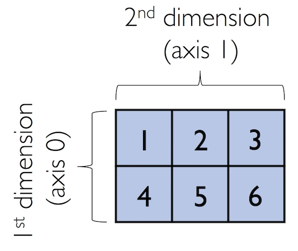
By default, NumPy infers the type of the array upon construction. Since we passed Python integers to the array, the ndarray object ary2d should be of type int64 on a 64-bit machine, which we can confirm by accessing the dtype attribute:
默认情况下,NumPy在构造时推断数组的类型。由于我们将Python整数传递给数组,因此ndarray对象ary2d在64位机器上的类型应该是int64,我们可以通过访问dtype属性来确认:
In:
python
ary2d.dtypeOut:
python
dtype('int64')If we want to construct NumPy arrays of different types, we can pass an argument to the dtype parameter of the array function, for example np.int32, to create 32-bit arrays. For a full list of supported data types, please refer to the official NumPy documentation. Once an array has been constructed, we can downcast or recast its type via the astype method as shown in the following examples:
如果我们想构造不同类型的NumPy数组,我们可以向数组函数的dtype参数传递一个参数,例如np.int32,以创建32位数组。有关支持的数据类型的完整列表,请参阅NumPy官方文档。构造完数组后,我们可以通过astype方法向下转换或重铸其类型,如下例所示:
In:
python
int32_ary = ary2d.astype(np.int32)
int32_ary
Out:
python
array([[1, 2, 3],
       [4, 5, 6]], dtype=int32)
In:
python
float32_ary = ary2d.astype(np.float32)
float32_ary
Out:
python
array([[1., 2., 3.],
       [4., 5., 6.]], dtype=float32)
In:
python
float32_ary.dtypeOut:
python
dtype('float32')In:
python
ary2d.itemsizeOut:
python
8The code snippet above returned 8, which means that each element in the array (remember that ndarrays are homogeneous) takes up 8 bytes in memory. This result makes sense since the array ary2d has type int64 (64-bit integer), which we determined earlier, and 8 bits equals 1 byte. (Note that 'int64' is just a shorthand for np.int64.)
上面的代码片段返回了8,这意味着数组中的每个元素(记住ndarray是同构的)在内存中占用8个字节。这个结果是有道理的,因为数组ary2d的类型为int64(64位整数),这是我们之前确定的,8位等于1字节。(请注意,"int64"只是np.int64的简写。)
To return the number of elements in an array, we can use the size attribute, as shown below:
要返回数组中的元素数量,我们可以使用size属性,如下所示:
And the number of dimensions of our array (Intuitively, you may think of dimensions as the rank of a tensor) can be obtained via the ndim attribute:
我们数组的维数(直观上,你可以把维数看作张量的秩)可以通过ndim属性获得:
In:
python
ary2dOut:
python
array([[1, 2, 3],
       [4, 5, 6]])
In:
python
ary2d.ndimOut:
python
2If we are interested in the number of elements along each array dimension (in the context of NumPy arrays, we may also refer to them as axes ), we can access the shape attribute as shown below:
如果我们对每个数组维度上的元素数量感兴趣(在NumPy数组的上下文中,我们也可以将它们称为轴),我们可以访问shape属性,如下所示:
In:
python
len(ary2d.shape)Out:
The shape is always a tuple; in the code example above, the two-dimensional ary object has two rows and three columns, (2, 3), if we think of it as a matrix representation.
形状总是一个元组;在上面的代码示例中,如果我们把二维ary对象看作矩阵表示,它有两行三列(2,3)。
Conversely, the shape (an object of type tuple) of a one-dimensional array only contains a single value:
相反,一维数组的形状(元组类型的对象)只包含一个值:
In:
python
np.array([1., 2., 3.]).shapeOut:
python
(3,)4.2: NumPy Array Construction and Indexing
Array Construction Routines
This section provides a non-comprehensive list of array construction functions. Simple yet useful functions exist to construct arrays containing ones or zeros:
本节提供了一个不全面的数组构造函数列表。存在简单但有用的函数来构造包含1或0的数组:
In:
python
np.ones((3, 4), dtype=np.int)Out:
python
array([[1, 1, 1, 1],
       [1, 1, 1, 1],
       [1, 1, 1, 1]])
In:
python
np.zeros((3, 3))Out:
python
array([[0., 0., 0.],
       [0., 0., 0.],
       [0., 0., 0.]])
说明 :输出中的
0.是浮点数0.0的简写形式。在 Python/NumPy 中,数字后加小数点表示这是一个浮点数(float)而非整数(int)。np.zeros()默认创建float64类型的数组,因此显示为0.而不是0。We can use these functions to create arrays with arbitrary values, e.g., we can create an array containing the values 99 as follows:
我们可以使用这些函数创建具有任意值的数组,例如,我们可以创建一个包含值99的数组,如下所示:
In:
python
np.zeros((3, 3)) + 99Out:
python
array([[99., 99., 99.],
       [99., 99., 99.],
       [99., 99., 99.]])
Creating arrays of ones or zeros can also be useful as placeholder arrays, in cases where we do not want to use the initial values for computations but want to fill it with other values right away. If we do not need the initial values (for instance, '0.' or '1.'), there is also numpy.empty, which follows the same syntax as numpy.ones and np.zeros. However, instead of filling the array with a particular value, the empty function creates the array with non-sensical values from memory. We can think of zeros as a function that creates the array via empty and then sets all its values to 0. -- in practice, a difference in speed is not noticeable, though.
在我们不想使用初始值进行计算但想立即用其他值填充的情况下,创建一个或零的数组也可以用作占位符数组。如果我们不需要初始值(例如"0."或"1."),还有numpy.empty,它遵循与numpy.ones和np.zeros相同的语法。但是,空函数不是用特定值填充数组,而是从内存中创建具有非意义值的数组。我们可以将零视为一个函数,它通过空创建数组,然后将其所有值设置为0。然而,在实践中,速度的差异并不明显。
NumPy also comes with functions to create identity matrices and diagonal matrices as ndarrays that can be useful in the context of linear algebra -- a topic that we will explore later in this article.
NumPy还附带了创建单位矩阵和对角矩阵作为ndarray的函数,这在线性代数的背景下非常有用------我们将在本文稍后探讨这个话题。
In:
python
np.eye(3)Out:
python
array([[1., 0., 0.],
       [0., 1., 0.],
       [0., 0., 1.]])
In:
python
np.diag((1, 2, 3))Out:
python
array([[1, 0, 0],
       [0, 2, 0],
       [0, 0, 3]])
Lastly, I want to mention two very useful functions for creating sequences of numbers within a specified range, namely, arange and linspace. NumPy's arange function follows the same syntax as Python's range objects: If two arguments are provided, the first argument represents the start value and the second value defines the stop value of a half-open interval:
最后,我想提到两个非常有用的函数,用于在指定范围内创建数字序列,即arange和linspace。NumPy的range函数遵循与Python的range对象相同的语法:如果提供了两个参数,则第一个参数表示半开区间的起始值,第二个值定义半开区间的停止值:
In:
python
np.arange(4, 10)Out:
python
array([4, 5, 6, 7, 8, 9])Notice that arange also performs type inference similar to the array function. If we only provide a single function argument, the range object treats this number as the endpoint of the interval and starts at 0:
请注意,arange也执行类似于数组函数的类型推断。如果我们只提供一个函数参数,range对象将此数字视为区间的端点,并从0开始:
In:
python
np.arange(5)Out:
python
array([0, 1, 2, 3, 4])Similar to Python's range, a third argument can be provided to define the step (the default step size is 1). For example, we can obtain an array of all uneven values between one and ten as follows:
与Python的范围类似,可以提供第三个参数来定义步长(默认步长为1)。例如,我们可以得到一个1到10之间所有不均匀值的数组,如下所示:
In:
python
np.arange(1., 11., 0.1)Out:
python
array([ 1. ,  1.1,  1.2,  1.3,  1.4,  1.5,  1.6,  1.7,  1.8,  1.9,  2. ,
        2.1,  2.2,  2.3,  2.4,  2.5,  2.6,  2.7,  2.8,  2.9,  3. ,  3.1,
        3.2,  3.3,  3.4,  3.5,  3.6,  3.7,  3.8,  3.9,  4. ,  4.1,  4.2,
        4.3,  4.4,  4.5,  4.6,  4.7,  4.8,  4.9,  5. ,  5.1,  5.2,  5.3,
        5.4,  5.5,  5.6,  5.7,  5.8,  5.9,  6. ,  6.1,  6.2,  6.3,  6.4,
        6.5,  6.6,  6.7,  6.8,  6.9,  7. ,  7.1,  7.2,  7.3,  7.4,  7.5,
        7.6,  7.7,  7.8,  7.9,  8. ,  8.1,  8.2,  8.3,  8.4,  8.5,  8.6,
        8.7,  8.8,  8.9,  9. ,  9.1,  9.2,  9.3,  9.4,  9.5,  9.6,  9.7,
        9.8,  9.9, 10. , 10.1, 10.2, 10.3, 10.4, 10.5, 10.6, 10.7, 10.8,
       10.9])
The linspace function is especially useful if we want to create a particular number of evenly spaced values in a specified half-open interval:
如果我们想在指定的半开区间中创建特定数量的均匀间隔值,linspace函数尤其有用:
In:
python
np.linspace(6., 15., num=10)Out:
python
array([ 6., 7., 8., 9., 10., 11., 12., 13., 14., 15.])Array Indexing
In this section, we will go over the basics of retrieving NumPy array elements via different indexing methods. Simple NumPy indexing and slicing works similar to Python lists, which we will demonstrate in the following code snippet, where we retrieve the first element of a one-dimensional array:
在本节中,我们将介绍通过不同索引方法检索NumPy数组元素的基础知识。简单的NumPy索引和切片的工作原理类似于Python列表,我们将在以下代码片段中演示,其中我们检索一维数组的第一个元素:
In:
python
ary = np.array([1, 2, 3])
ary[0]
Out:
python
1Also, the same Python semantics apply to slicing operations. The following example shows how to fetch the first two elements in ary:
同样的Python语义也适用于切片操作。以下示例显示了如何获取ary中的前两个元素:
In:
python
ary[0:3] # equivalent to ary[0:2]Out:
python
array([1, 2, 3])If we work with arrays that have more than one dimension or axis, we separate our indexing or slicing operations by commas as shown in the series of examples below:
如果我们使用具有多个维度或轴的数组,我们可以用逗号分隔索引或切片操作,如下面的一系列示例所示:
In:
python
ary = np.array([[1, 2, 3],
                [4, 5, 6]])
ary[0, -2] # first row, second from last element
Out:
python
2In:
python
ary[-1, -1] # lower rightOut:
python
6In:
python
ary[1, 1] # first row, second columnOut:
python
5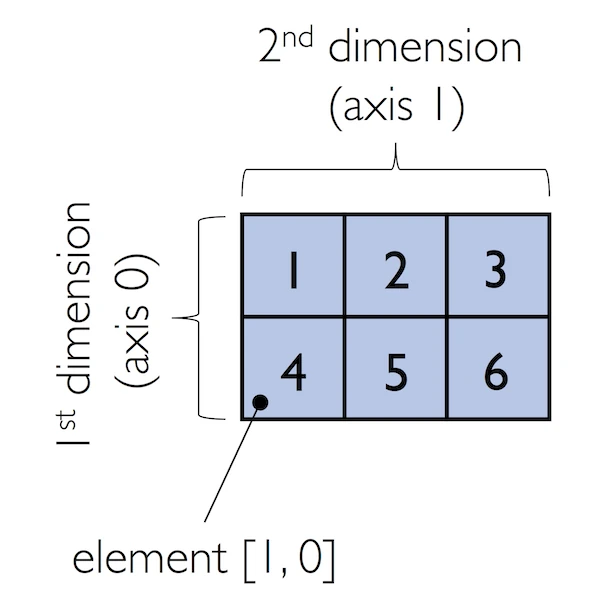
In:
python
ary[:, 0] # entire first columnOut:
In:
python
ary[:, :2] # first two columnsOut:
4.3: NumPy Array Math and Universal Functions
Array Math and Universal Functions
In the previous sections, you learned how to create NumPy arrays and how to access different elements in an array. It is about time that we introduce one of the core features of NumPy that makes working with ndarray so efficient and convenient: vectorization. While we typically use for-loops if we want to perform arithmetic operations on sequence-like objects, NumPy provides vectorized wrappers for performing element-wise operations implicitly via so-called ufuncs -- "ufuncs" is short for universal functions.
在前面的部分中,您学习了如何创建NumPy数组以及如何访问数组中的不同元素。现在是时候介绍NumPy的一个核心特性了,它使使用ndarray变得如此高效和方便:矢量化。虽然我们通常使用for循环来对类序列对象执行算术运算,但NumPy提供了矢量化包装器,用于通过所谓的ufuncs隐式执行元素操作------"ufuncs"是通用函数的缩写。
As of this writing, there are more than 60 ufuncs available in NumPy; ufuncs are implemented in compiled C code and very fast and efficient compared to vanilla Python. In this section, we will take a look at the most commonly used ufuncs, and I recommend you to check out the official documentation for a complete list.
在撰写本文时,NumPy中有60多个ufunc可用;ufuncs是用编译的C代码实现的,与普通Python相比非常快速高效。在本节中,我们将介绍最常用的ufunc,我建议您查看官方文档以获取完整列表。
To provide an example of a simple ufunc for element-wise addition, consider the following example, where we add a scalar (here: 1) to each element in a nested Python list:
为了提供一个用于元素添加的简单ufunc示例,请考虑以下示例,其中我们向嵌套Python列表中的每个元素添加一个标量(这里:1):
In:
python
lst = [[1, 2, 3],
       [4, 5, 6]] # 2d array
for row_idx, row_val in enumerate(lst):
    for col_idx, col_val in enumerate(row_val):
        lst[row_idx][col_idx] += 1
lst
Out:
python
[[2, 3, 4], [5, 6, 7]]This for-loop approach is very verbose, and we could achieve the same goal more elegantly using list comprehensions:
这种for循环方法非常冗长,我们可以使用列表推导更优雅地实现同样的目标:
In:
python
lst = [[1, 2, 3], [4, 5, 6]]
[[cell + 1 for cell in row] for row in lst]
Out:
python
[[2, 3, 4], [5, 6, 7]]We can accomplish the same using NumPy's ufunc for element-wise scalar addition as shown below:
我们可以使用NumPy的ufunc进行元素级标量加法,如下所示:
In:
python
ary = np.array([[1, 2, 3], [4, 5, 6]])
ary = np.add(ary, 1) # binary ufunc
ary
Out:
python
array([[2, 3, 4],
       [5, 6, 7]])
The ufuncs for basic arithmetic operations are add, subtract, divide, multiply, power, and exp (exponential). However, NumPy uses operator overloading so that we can use mathematical operators (+, -, /, *, and **) directly:
基本算术运算的ufuncs是加、减、除、乘、幂和exp(指数)。但是,NumPy使用运算符重载,因此我们可以直接使用数学运算符(+、-、/、和*):
In:
python
np.add(ary, 1)Out:
python
array([[3, 4, 5],
       [6, 7, 8]])
In:
python
ary + 1Out:
python
array([[3, 4, 5],
       [6, 7, 8]])
In:
python
np.power(ary, 2)Out:
python
array([[ 4,  9, 16],
       [25, 36, 49]])
In:
python
np.power(ary, 2)Out:
python
array([[ 4,  9, 16],
       [25, 36, 49]])
Above, we have seen examples of binary ufuncs, which are ufuncs that take two arguments as an input. In addition, NumPy implements several useful unary ufuncs, such as log (natural logarithm), log10 (base-10 logarithm), and sqrt (square root):
上面,我们看到了二进制ufunc的示例,这是一种将两个参数作为输入的ufunc。此外,NumPy实现了几个有用的一元ufunc,如log(自然对数)、log10(以10为底的对数)和sqrt(平方根):
In:
python
np.sqrt(ary)Out:
python
array([[1.41421356, 1.73205081, 2.        ],
       [2.23606798, 2.44948974, 2.64575131]])
Often, we want to compute the sum or product of array element along a given axis. For this purpose, we can use a ufunc's reduce operation. By default, reduce applies an operation along the first axis (axis=0). In the case of a two-dimensional array, we can think of the first axis as the rows of a matrix. Thus, adding up elements along rows yields the column sums of that matrix as shown below:
通常,我们想计算沿给定轴的数组元素的和或积。为此,我们可以使用ufunc的reduce操作。默认情况下,reduce沿第一个轴(轴=0)应用操作。在二维数组的情况下,我们可以将第一轴视为矩阵的行。因此,沿行添加元素会得到该矩阵的列和,如下所示:
In:
python
ary = np.array([[1, 2, 3],
                [4, 5, 6]]) # rolling over the 1st axis, axis 0
np.add.reduce(ary, axis=0)
关于
reduce的解释英文含义 :
reduce的英文意思是"减少、缩减、合并",指将多个元素通过某种操作合并成更少的元素(通常是一个)。在 NumPy 中的含义 :
np.add.reduce()是一个聚合操作 ,它会沿着指定的轴对数组元素反复应用加法,把多个数值"压缩"成一个结果。工作原理:
np.add.reduce(ary, axis=0)会沿着第0轴(行方向)进行聚合- 对于二维数组,这意味着将所有行相加,得到每列的总和
- 例如:
[[1,2,3], [4,5,6]]→[1+4, 2+5, 3+6]→[5, 7, 9]类比理解 :就像把多层积木压扁成一层,通过"相加"的方式将多个数值"压缩"成一个数值。
Out:
python
array([5, 7, 9])To compute the row sums of the array above, we can specify axis=1:
为了计算上述数组的行和,我们可以指定axis=1:
In:
python
np.add.reduce(ary, axis=1) # row sumsOut:
python
array([ 6, 15])While it can be more intuitive to use reduce as a more general operation, NumPy also provides shorthands for specific operations such as product and sum. For example, sum(axis=0) is equivalent to add.reduce:
虽然将reduce用作更通用的操作可能更直观,但NumPy还为特定的操作(如乘积和总和)提供了简写。例如,sum(axis=0)等价于add.reduce:
In:
python
ary.sum(axis=0) # column sumsOut:
python
array([5, 7, 9])In:
python
ary.sum(axis=1) # row sumsOut:
python
array([ 6, 15])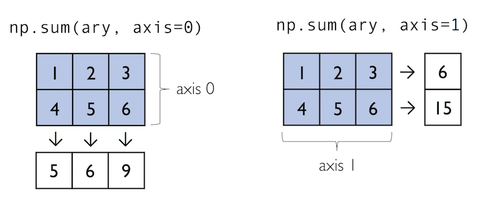
As a word of caution, keep in mind that product and sum both compute the product or sum of the entire array if we do not specify an axis:
作为警告,请记住,如果我们不指定轴,乘积和总和都会计算整个数组的乘积或总和:
In:
python
ary.sum()Out:
python
21Other useful unary ufuncs are:其他有用的一元ufunc是:
np.mean(computes arithmetic mean or average)np.mean(计算算术平均值或平均值)np.std(computes the standard deviation)np.std(计算标准偏差)np.var(computes variance)np.var(计算方差)np.sort(sorts an array)np.sort(对数组进行排序)np.argsort(returns indices that would sort an array)np.argsort(返回对数组进行排序的索引)np.min(returns the minimum value of an array)np.min(返回数组的最小值)np.max(returns the maximum value of an array)np.max(返回数组的最大值)np.argmin(returns the index of the minimum value)np.argmin(返回最小值的索引)np.argmax(returns the index of the maximum value)np.argmax(返回最大值的索引)np.array_equal(checks if two arrays have the same shape and elements)np.array_equal(检查两个数组是否具有相同的形状和元素)
4.4: NumPy Broadcasting
Broadcasting
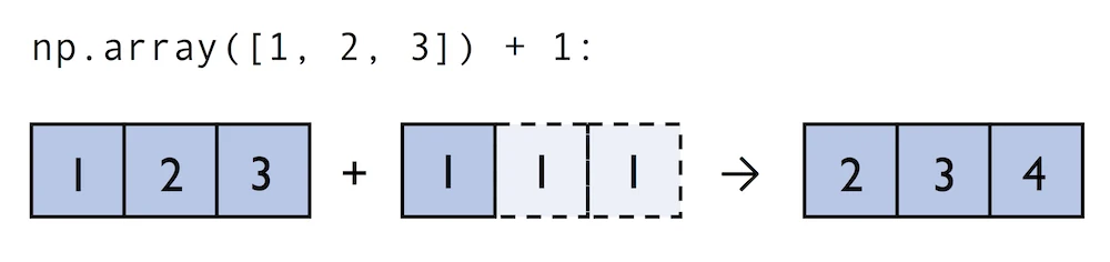
A topic we glanced over in the previous section is broadcasting. Broadcasting allows us to perform vectorized operations between two arrays even if their dimensions do not match by creating implicit multidimensional grids. You already learned about ufuncs in the previous section where we performed element-wise addition between a scalar and a multidimensional array, which is just one example of broadcasting.
我们在上一节中浏览过的一个主题是广播。广播允许我们通过创建隐式多维网格在两个数组之间执行矢量化操作,即使它们的维度不匹配。在上一节中,您已经了解了ufuncs,我们在标量和多维数组之间执行了元素相加,这只是广播的一个示例。
Naturally, we can also perform element-wise operations between arrays of equal dimensions:
当然,我们也可以在等维数组之间执行元素操作:
In contrast to what we are used from linear algebra, we can also add arrays of different shapes. In the example above, we will add a one-dimensional to a two-dimensional array, where NumPy creates an implicit multidimensional grid from the one-dimensional array ary1:
与线性代数中使用的相反,我们还可以添加不同形状的数组。在上面的例子中,我们将向二维数组添加一个一维数组,其中NumPy从一维数组ary1创建一个隐式多维网格:
In:
python
ary = np.array([1, 2, 3])
ary + 1
Out:
python
array([2, 3, 4])In:
python
ary + np.array([1, 1, 1])Out:
python
array([2, 3, 4])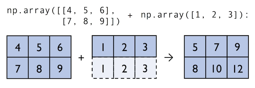
In:
python
ary2 = np.array([[4, 5, 6],
                 [7, 8, 9]])
ary2 + ary
Out:
python
array([[ 5,  7,  9],
       [ 8, 10, 12]])
4.5: NumPy Advanced Indexing -- Memory Views and Copies
Advanced Indexing -- Memory Views and Copies
In the previous sections, we have used basic indexing and slicing routines. It is important to note that basic integer-based indexing and slicing create so-called views of NumPy arrays in memory. Working with views can be highly desirable since it avoids making unnecessary copies of arrays to save memory resources. To illustrate the concept of memory views, let us walk through a simple example where we access the first row in an array, assign it to a variable, and modify that variable:
在前面的部分中,我们使用了基本的索引和切片例程。值得注意的是,基本的基于整数的索引和切片在内存中创建了所谓的NumPy数组视图。使用视图可能是非常可取的,因为它避免了制作不必要的数组副本以节省内存资源。为了说明内存视图的概念,让我们通过一个简单的例子来演示,在这个例子中,我们访问数组中的第一行,将其赋值给一个变量,并修改该变量:
In:
python
ary = np.array([[1, 2, 3],
                [4, 5, 6]])
first_row = ary[0]

first_row
Out:
python
array([1, 2, 3])In:
python
first_row += 99Out:
As expected, first_row was modified, now containing the original values in the first row incremented by 99:
Out:正如预期的那样,first_row被修改了,现在第一行中的原始值增加了99:
In:
python
first_rowOut:
python
array([100, 101, 102])Note, however, that the original array was modified as well:
但是请注意,原始数组也被修改了:
In:
python
aryOut:
python
array([[100, 101, 102],
       [  4,   5,   6]])
As we saw in the example above, changing the value of first_row also affected the original array. The reason for this is that ary[0] created a view of the first row in ary, and its elements were then incremented by 99. The same concept applies to slicing operations:
正如我们在上面的示例中看到的,更改first_row的值也会影响原始数组。原因是ary0创建了ary中第一行的视图,然后将其元素递增99。同样的概念也适用于切片操作:
In:
python
ary = np.array([[1, 2, 3],
                [4, 5, 6]])
first_row = ary[1:3]
first_row += 99
ary
简单理解
ary[1:3]
ary[1:3]可以看成:从第 1 行开始取,一直取到第 3 行前面为止。
这里虽然数组只有第 0 行和第 1 行,没有第 2 行,但这不会报错 ,因为切片和直接索引不一样:
- 直接索引 :如
ary[2],如果第 2 行不存在,就会报越界错误。- 切片 :如
ary[1:3],即使终点超过范围,也只会"取到能取到的部分",不会报错。所以这里实际拿到的就是:第 1 行及其后能取到的行 ,结果只有一行。
另外,二维数组里写
ary[1:3]时,默认表示:ary[1:3, :],也就是"取这些行,列全部保留"。Out:
python
array([[  1,   2,   3],
       [103, 104, 105]])
In:
python
ary = np.array([[1, 2, 3],
                [4, 5, 6]])
center_col = ary[:, 2]
center_col += 99
ary
Out:
python
array([[  1,   2, 102],
       [  4,   5, 105]])
If we are working with NumPy arrays, it is always important to be aware that slicing creates views -- sometimes it is desirable since it can speed up our code by avoiding to create unnecessary copies in memory. However, in certain scenarios we want force a copy of an array; we can do this via the copy method as shown below:
如果我们使用NumPy数组,重要的是要意识到切片会创建视图------有时这是可取的,因为它可以通过避免在内存中创建不必要的副本来加速我们的代码。然而,在某些情况下,我们希望强制复制数组;我们可以通过如下所示的复制方法来实现这一点:
In:
python
ary = np.array([[1, 2, 3],
                [4, 5, 6]])
first_row = ary[0].copy()
first_row += 99
In:
python
first_rowOut:
python
array([100, 101, 102])In:
python
aryOut:
python
array([[1, 2, 3],
       [4, 5, 6]])
Fancy Indexing
In addition to basic single-integer indexing and slicing operations, NumPy supports advanced indexing routines called fancy indexing. Via fancy indexing, we can use tuple or list objects of non-contiguous integer indices to return desired array elements. Since fancy indexing can be performed with non-contiguous sequences, it cannot return a view -- a contiguous slice from memory. Thus, fancy indexing always returns a copy of an array -- it is important to keep that in mind. The following code snippets show some fancy indexing examples:
除了基本的单整数索引和切片操作外,NumPy还支持称为花式索引的高级索引例程。通过花哨的索引,我们可以使用非连续整数索引的元组或列表对象来返回所需的数组元素。由于可以使用非连续序列执行花哨的索引,因此它不能返回视图------内存中的连续切片。因此,花哨的索引总是返回数组的副本------记住这一点很重要。以下代码片段显示了一些花哨的索引示例:
In:
python
ary = np.array([[1, 2, 3],
                [4, 5, 6]])
ary[:, [0, 2]] # first and and last column
Out:
python
array([[1, 3],
       [4, 6]])
In:
python
this_is_a_copy = ary[:, [0, 2]]
this_is_a_copy += 99
Note that the values in this_is_a_copy were incremented as expected:
请注意,this_is_a_copy中的值按预期递增:
In:
python
this_is_a_copyOut:
python
array([[100, 102],
       [103, 105]])
However, the contents of the original array remain unaffected:
但是,原始数组的内容不受影响:
In:
python
aryOut:
python
array([[1, 2, 3],
       [4, 5, 6]])
NumPy 的视图(View)与副本(Copy):为什么 Fancy Indexing 不同?
触及 NumPy 高性能核心机制的一个问题:为什么切片能返回视图,而 fancy indexing 必须返回副本?下面从内存布局角度"深入浅出"讲清楚。
一、核心概念:ndarray 的两个部分
一个 NumPy 数组在内存中由两个东西组成:
- 数据缓冲区(Data Buffer):一块连续的内存,真正存放数字。
- 元信息(Metadata) :描述"如何解读这块内存",包括:
shape(形状)strides(步长:在每个维度上,走一步要跳过多少字节)dtype(数据类型)- 指向数据缓冲区起始位置的指针(
offset)关键点 :只要"一段连续内存 + 一组规则(strides + offset)"能够描述出你想要的元素,NumPy 就能创建一个视图(View)------它共享同一块数据缓冲区,只是换了一套解读规则。
二、内存图:原始数组
pythonimport numpy as np ary = np.array([[1, 2, 3], [4, 5, 6], [7, 8, 9]])内存中的数据缓冲区(C 顺序,行优先,连续排列):
内存地址(字节): 0    8    16   24   32   40   48   56   64
数据缓冲区:     [ 1 ][ 2 ][ 3 ][ 4 ][ 5 ][ 6 ][ 7 ][ 8 ][ 9 ]
索引位置:         0    1    2    3    4    5    6    7    8

元信息:
  shape   = (3, 3)
  strides = (24, 8)   # 下移一行跳 24 字节(3个int64), 右移一列跳 8 字节
  offset  = 0
三、切片
ary[:, 2]为什么能返回视图?
pythoncenter_col = ary[:, 2] # -> array([3, 6, 9])我们要的元素是
3, 6, 9,它们在缓冲区中的索引是2, 5, 8。看它们的字节地址:
16, 40, 64------ 它们间隔相等(每次 +24 字节)!
内存地址(字节): 0    8    16   24   32   40   48   56   64
数据缓冲区:     [ 1 ][ 2 ][ 3 ][ 4 ][ 5 ][ 6 ][ 7 ][ 8 ][ 9 ]
                          ↑              ↑              ↑
center_col 取:            3              6              9
                     (offset=16)     (+24)          (+24)
因此可以用一套简单规则描述:
center_col 的元信息(视图): shape = (3,) strides = (24,) # 每走一步跳 24 字节 offset = 16 # 从第 16 字节开始 ★ 数据缓冲区 = 与 ary 共享(同一块内存)因为只需要 offset + 固定 stride 就能定位到全部所需元素,NumPy 无需复制任何数据,直接返回视图。这也是为什么修改视图会影响原数组:
pythoncenter_col[0] = 100 print(ary[0, 2]) # 100 <- 原数组被改变!
四、Fancy Indexing
ary[:, [0, 2]]为什么必须返回副本?
pythonpicked = ary[:, [0, 2]] # 取第 0 列 和 第 2 列 # -> array([[1, 3], # [4, 6], # [7, 9]])我们要的元素在缓冲区的索引是:
0, 2, 3, 5, 6, 8。
内存地址(字节): 0    8    16   24   32   40   48   56   64
数据缓冲区:     [ 1 ][ 2 ][ 3 ][ 4 ][ 5 ][ 6 ][ 7 ][ 8 ][ 9 ]
                 ↑         ↑    ↑         ↑    ↑         ↑
需要的元素:      1         3    4         6    7         9
字节地址:        0        16   24        40   48        64
相邻间隔:            +16     +8    +16      +8    +16
                ↑ 不规则的跳跃步长 ↑
问题来了 :这些地址的间隔是
+16, +8, +16, +8, +16------不是一个固定的 stride!无论怎么设置
offset和strides,都无法用一个统一的规则把这些非连续、非等间距的元素描述出来。既然规则表达不了,NumPy 只能:老老实实把这些元素一个个复制出来,放进一块全新的、连续的内存里。
新分配的连续内存(副本):
内存地址(字节): 0    8    16   24   32   40
数据缓冲区:     [ 1 ][ 3 ][ 4 ][ 6 ][ 7 ][ 9 ]

  shape   = (3, 2)
  strides = (16, 8)
  offset  = 0
  ★ 全新的独立内存(与 ary 不共享)
所以修改 fancy indexing 的结果不会影响原数组:
pythonpicked[0, 0] = 100 print(ary[0, 0]) # 1 <- 原数组不受影响!
五、一句话总结
操作类型 能否用 offset + 固定 strides描述?结果 切片 ary[:, 2]✅ 等间距,可以 视图 (共享内存) Fancy indexing ary[:, [0,2]]❌ 间距不规则,做不到 副本 (独立内存) 根本原因 :视图必须依赖"连续内存 + 规则的 strides"来定位元素;而 fancy indexing 用任意的索引列表选取元素,这些元素在内存中通常非连续、非等间距,无法用统一规则表达,因此 NumPy 必须复制数据到一块新内存中。
💡 记忆锚点
- 切片(slicing) = "改一套解读规则" → 视图
- 花式索引(fancy indexing) = "挑好的搬到新家" → 副本
这也是为什么 fancy indexing 更灵活(能任意挑选、重排、重复元素),但代价是额外的内存分配与拷贝开销。
Boolean Masks for Indexing
Finally, we can also use Boolean masks for indexing -- that is, arrays of True and False values. Consider the following example, where we return all values in the array that are greater than 3:
最后,我们还可以使用布尔掩码进行索引,即True和False值的数组。考虑以下示例,我们返回数组中大于3的所有值:
In:
python
ary = np.array([[1, 2, 3],
                [4, 5, 6]])
greater3_mask = ary > 3
greater3_mask
Out:
python
array([[False, False, False],
       [ True,  True,  True]])
Using these masks, we can select elements given our desired criteria:
使用这些掩码,我们可以根据所需的标准选择元素:
In:
python
ary[greater3_mask]Out:
python
array([4, 5, 6])We can also chain different selection criteria using the logical and operator & or the logical or operator |. The example below demonstrates how we can select array elements that are greater than 3 and divisible by 2:
我们还可以使用逻辑和运算符&或逻辑或运算符|来链接不同的选择标准。下面的示例演示了如何选择大于3且可被2整除的数组元素:
In:
python
(ary > 3) & (ary % 2 == 0)Out:
python
array([[False, False, False],
       [ True, False,  True]])
Similar to the previous example, we can use this boolean array as a mask for selecting the respective elements from the array:
与前面的例子类似,我们可以使用这个布尔数组作为掩码,从数组中选择相应的元素:
In:
python
ary[(ary > 3) & (ary % 2 == 0)]Out:
python
array([4, 6])Note that indexing using Boolean arrays is also considered "fancy indexing" and thus returns a copy of the array.
请注意,使用布尔数组进行索引也被认为是"花哨的索引",因此会返回数组的副本。
In:
python
ary = np.array([[7, 2, 5],
                [1, 4, 9]])


print(ary % 2 == 0)

print(ary[ary % 2 == 0])
Out:
python
[[False  True False]
 [False  True False]]
[2 4]
NumPy 布尔索引(Boolean Masking)为什么结果总是一维
核心结论:ndarray 底层永远是一条连续的直线,维度只是「解读方式」。布尔索引沿这条直线扫描,把
True位置的元素按顺序捡出------因为选中的数量和分布不规则,无法拼成矩形,所以结果只能是一维。
1. ndarray 在内存里长什么样
一个 NumPy 数组在内存中其实是一整块连续的一维缓冲区(buffer),再加上一份「怎么解读这块内存」的元信息。
pythonary = np.array([[7, 2, 5], [1, 4, 9]])它在内存里实际是这样存的(默认 C order,行优先):
内存地址递增 →
┌───┬───┬───┬───┬───┬───┐
│ 7 │ 2 │ 5 │ 1 │ 4 │ 9 │   ← 真正的数据,一条直线
└───┴───┴───┴───┴───┴───┘
  0   1   2   3   4   5     ← 线性偏移(flat index)
那个「二维」的形态,只是靠
shape=(2,3)和strides这些元信息「投影」出来的:
逻辑视图              内存现实
[[7, 2, 5],          7 2 5 1 4 9
 [1, 4, 9]]          (本质是一条线)
二维只是「戴上的一副眼镜」,底层永远是一条直线。
2. 布尔掩码在做什么
pythonmask = ary % 2 == 0 # [[False True False] # [False True False]]关键点:掩码在逻辑上 是二维,但底层它同样是一条直线,和
ary的元素一一对应:
ary  的内存:   7      2      5      1      4      9
mask 的内存: False  True   False  False  True   False
偏移:      0      1      2      3      4      5
当你执行
ary[mask]时,NumPy 做的事情非常简单粗暴:沿着这条直线从头走到尾,mask 是True的位置,就把对应的元素捡出来,按走过的顺序依次放进一个新的一维缓冲区。
遍历过程:
偏移0: mask=False → 跳过
偏移1: mask=True  → 捡出 2 ┐
偏移2: mask=False → 跳过  │
偏移3: mask=False → 跳过  ├→ 收集
偏移4: mask=True  → 捡出 4 ┘
偏移5: mask=False → 跳过

结果缓冲区: [2, 4]
3. 为什么结果必须是一维
核心原因:被选中的元素个数是不确定的,而且它们在原数组里的分布是任意的。
设想一下,如果 NumPy 想保留二维形状,它会遇到矛盾:
[[False  True False]      第一行选中 1 个
 [ True  True False]]     第二行选中 2 个
第一行捡出 1 个,第二行捡出 2 个 ------ 你没法把它们拼回一个规整的矩形(矩形要求每行元素数相同)。ndarray 必须是规整的矩形/长方体 (每个维度长度固定),它无法表示「参差不齐」的形状。唯一能确定、且永远合法的形状,就是一维:不管选中几个,排成一条线总是成立的。所以 NumPy 干脆规定:布尔掩码索引一律返回一维数组。
任意形状 + 任意掩码 ──布尔索引──▶ 一维结果(把选中的元素拉直排列)
4. 复合掩码例子
pythonary = np.array([[1, 2, 3], [4, 5, 6]]) ary[(ary > 3) & (ary % 2 == 0)] # array([4, 6])先算复合掩码(
&是逐元素与):
内存:        1      2      3      4      5      6
>3:        F      F      F      T      T      T
%2==0:     F      T      F      T      F      T
&:         F      F      F      T      F      T   ← 最终 mask
沿直线捡出 mask 为 True 的:偏移3 的
4、偏移5 的6:
array([4, 6])
5. 对照记忆点
- 布尔掩码
ary[mask]→ 结果拉平成一维(数量不定)。- 切片
ary[0:2, 1:3]→ 保留维度(因为切片是规整的矩形区域)。- 整数数组索引
ary[[0,1],[2,0]]→ 结果形状跟着索引数组的形状走(另一套规则)。验证技巧 :对比
ary[mask]和ary.ravel()[mask.ravel()],两者结果完全一致------这正说明布尔索引就是在扁平化的缓冲区上操作。
4.6: Random Number Generators
Random Number Generators
In machine learning and deep learning, we often have to generate arrays of random numbers -- for example, the initial values of our model parameters before optimization. NumPy has a random subpackage to create random numbers and samples from a variety of distributions conveniently. Again, I encourage you to browse through the more comprehensive numpy.random documentation for a complete list of functions for random sampling.
在机器学习和深度学习中,我们通常必须生成随机数数组,例如优化前模型参数的初始值。NumPy有一个随机子包,可以方便地从各种分布中创建随机数和样本。我再次鼓励您浏览更全面的numpy.random文档,以获取随机采样函数的完整列表。
To provide a brief overview of the pseudo-random number generators that we will use most commonly, let's start with drawing a random sample from a uniform distribution:
为了简要概述我们最常用的伪随机数生成器,让我们从均匀分布中提取随机样本开始:
In:
python
np.random.seed(123)
np.random.rand(3)
Out:
python
array([0.69646919, 0.28613933, 0.22685145])In the code snippet above, we first seeded NumPy's random number generator. Then, we drew three random samples from a uniform distribution via random.rand in the half-open interval [0, 1). I highly recommend the seeding step in practical applications as well as in research projects, since it ensures that our results are reproducible. If we run our code sequentially -- for example, if we execute a Python script -- it should be sufficient to seed the random number generator only once at the beginning to enforce reproducible outcomes between different runs. However, it is often useful to create separate RandomState objects for various parts of our code, so that we can test methods of functions reliably in unit tests. Working with multiple, separate RandomState objects can also be useful if we run our code in non-sequential order -- for example if we are experimenting with our code in interactive sessions or Jupyter Notebook environments.
在上面的代码片段中,我们首先为NumPy的随机数生成器接种种子。然后,我们通过random.rand在半开区间[0,1)中从均匀分布中提取了三个随机样本。我强烈建议在实际应用和研究项目中使用种子步骤,因为它可以确保我们的结果是可重复的。如果我们按顺序运行代码,例如,如果我们执行Python脚本,那么在开始时只给随机数生成器种子一次就足以在不同运行之间强制执行可重复的结果。但是,为代码的各个部分创建单独的RandomState对象通常很有用,这样我们就可以在单元测试中可靠地测试函数的方法。如果我们以非顺序运行代码(例如,如果我们正在交互式会话或Jupyter Notebook环境中试验我们的代码。
The example below shows how we can use a RandomState object to create the same results that we obtained via np.random.rand in the previous code snippet:
下面的示例显示了如何使用RandomState对象创建与我们在前面的代码片段中通过np.random.rand获得的结果相同的结果:
In:
python
rng2 = np.random.RandomState(seed=531)
rng2.rand(3)
Out:
python
array([0.68980796, 0.35494577, 0.94994208])Also, the NumPy developer community developed new random number generation method in recent versions of NumPy. For more details, please see the new random Generator documentation:
此外,NumPy开发人员社区在最新版本的NumPy中开发了新的随机数生成方法。有关更多详细信息,请参阅新的随机生成器文档:
In:
python
rng2 = np.random.default_rng(seed=123)
rng2.random(3)
Out:
python
array([0.68235186, 0.05382102, 0.22035987])4.7: Reshaping NumPy Arrays
Reshaping Arrays
In practice, we often run into situations where existing arrays do not have the right shape to perform certain computations. As you might remember from the beginning of this article, the size of NumPy arrays is fixed. Fortunately, this does not mean that we have to create new arrays and copy values from the old array to the new one if we want arrays of different shapes -- the size is fixed, but the shape is not. NumPy provides a reshape methods that allow us to obtain a view of an array with a different shape.
在实践中,我们经常遇到现有数组没有正确形状来执行某些计算的情况。您可能还记得,从本文开始,NumPy数组的大小是固定的。幸运的是,这并不意味着如果我们想要不同形状的数组,我们必须创建新的数组并将值从旧数组复制到新数组------大小是固定的,但形状不是。NumPy提供了一种整形方法,使我们能够获得具有不同形状的数组视图。
For example, we can reshape a one-dimensional array into a two-dimensional one using reshape as follows:
例如,我们可以使用reshape将一维数组重塑为二维数组,如下所示:
In:
python
ary1d = np.array([1, 2, 3, 4, 5, 6])
ary2d_view = ary1d.reshape(2, 3)
ary2d_view
Out:
python
array([[1, 2, 3],
       [4, 5, 6]])
The True value returned from np.may_share_memory indicates that the reshape operation returns a memory view, not a copy:
np.may_share_memory返回的True值表示整形操作返回的是内存视图,而不是副本:
In:
python
np.may_share_memory(ary2d_view, ary1d)Out:
python
TrueWhile we need to specify the desired elements along each axis, we need to make sure that the reshaped array has the same number of elements as the original one. However, we do not need to specify the number elements in each axis; NumPy is smart enough to figure out how many elements to put along an axis if only one axis is unspecified (by using the placeholder -1):
虽然我们需要沿每个轴指定所需的元素,但我们需要确保重塑后的数组具有与原始数组相同的元素数量。然而,我们不需要指定每个轴中的数字元素;NumPy足够聪明,可以在只有一个轴未指定的情况下(通过使用占位符-1)计算出沿一个轴放置多少个元素:
In:
python
ary1d.reshape(-1, 2)Out:
python
array([[1, 2],
       [3, 4],
       [5, 6]])
问题 2:占位符
-1的含义
-1的意思是:"这个轴的大小你(NumPy)自己算出来"。因为 reshape 前后元素总数必须相等,所以当你指定了其他轴的大小后,剩下这一个轴的大小其实是唯一确定的,不需要你手动算。
-1就是告诉 NumPy "帮我把这个数补上"。以
ary1d.reshape(-1, 2)为例:
- 总共有 6 个元素
- 你指定了第二个轴(列)是 2
- 那么行数 = 6 ÷ 2 = 3
所以结果是
(3, 2):
pythonarray([[1, 2], [3, 4], [5, 6]])
reshape(-1)就是把所有元素铺到一个轴上,等价于展平成一维。关键限制 :
-1只能出现一次 。如果你写reshape(-1, -1),NumPy 无法确定该怎么分配,会直接报错------因为方程有无穷多解。问题 3:
concatenate的 axis 到底怎么理解这个问题很常见,因为直觉容易把"沿 axis=0"理解成"横向拼",但实际正好相反。
先记住一个核心原则:
axis=N表示沿着第 N 个轴的方向"堆叠/延长",也就是让第 N 个维度的长度变大,其他维度长度保持不变。看你的例子。
ary = np.array([[1, 2, 3]])注意这里是两层方括号 ,所以它是一个二维数组,形状是(1, 3)------1 行 3 列:
        列0 列1 列2
行0:      1   2   3
axis=0(沿行方向延长)
axis=0是行这个维度。沿 axis=0 拼接,就是让行数增加 ,列数不变。两个(1, 3)拼起来,行数从 1 变成 2,结果是(2, 3):
pythonnp.concatenate((ary, ary), axis=0) # array([[1, 2, 3], # [1, 2, 3]])直观理解:把第二个数组摞在第一个数组下面。这就像叠盘子------一个个往下加。
        列0 列1 列2
行0:      1   2   3   ← 第一个 ary
行1:      1   2   3   ← 第二个 ary
axis=1(沿列方向延长)
axis=1是列这个维度。沿 axis=1 拼接,就是让列数增加 ,行数不变。两个(1, 3)拼起来,列数从 3 变成 6,结果是(1, 6):
pythonnp.concatenate((ary, ary), axis=1) # array([[1, 2, 3, 1, 2, 3]])直观理解:把第二个数组接在第一个数组右边。
        列0 列1 列2 列3 列4 列5
行0:      1   2   3   1   2   3
        └─第一个 ary─┘└─第二个 ary─┘
为什么容易搞反
很多人的直觉是:"0 是行,行不就是横着的一条吗?那沿 axis=0 应该横着拼呀。" 但
axis=0指的不是"沿着某一行内部移动",而是"沿着行编号增大的方向 ",也就是竖着往下走。换个记法可能更好记:
axis=N就是那个会变长的维度的下标。
axis=0→shape[0](行数)变大 → 竖向增长axis=1→shape[1](列数)变大 → 横向增长再验证一下形状规律:两个
(1, 3)拼接
axis=0:第 0 维相加1+1=2,第 1 维不变3→(2, 3)✓axis=1:第 0 维不变1,第 1 维相加3+3=6→(1, 6)✓约束 :除了要拼接的那个轴,其他所有轴的长度必须完全一致,否则拼不起来会报错。比如一个
(2, 3)和一个(2, 4)可以沿axis=1拼成(2, 7)(行数都是 2),但不能沿axis=0拼(列数 3 ≠ 4)。
We can, of course, also use reshape to flatten an array:
当然,我们也可以使用reshape来展平数组:
In:
python
ary = np.array([[[1, 2, 3],
                 [4, 5, 6]]])
ary.reshape(-1)
Out:
python
array([1, 2, 3, 4, 5, 6])Other methods for flattening arrays exist, namely flatten, which creates a copy of the array, and ravel, which creates a memory view like reshape:
还存在其他展平数组的方法,即展平,它创建数组的副本,以及拉威尔,它创建类似重塑的内存视图:
In:
python
ary.flatten()Out:
python
array([1, 2, 3, 4, 5, 6])In:
python
ary.ravel()Out:
python
array([1, 2, 3, 4, 5, 6])Sometimes, we are interested in merging different arrays. Unfortunately, there is no efficient way to do this without creating a new array, since NumPy arrays have a fixed size. While combining arrays should be avoided if possible -- for reasons of computational efficiency -- it is sometimes necessary. To combine two or more array objects, we can use NumPy's concatenate function as shown in the following examples:
有时,我们对合并不同的数组感兴趣。不幸的是,在不创建新数组的情况下,没有有效的方法可以做到这一点,因为NumPy数组的大小是固定的。虽然出于计算效率的原因,应尽可能避免组合数组,但有时这是必要的。要组合两个或多个数组对象,我们可以使用NumPy的concatenate函数,如下例所示:
In:
python
ary = np.array([1, 2, 3])
# stack along the first axis
np.concatenate((ary, ary))
Out:
python
array([1, 2, 3, 1, 2, 3])In:
python
ary = np.array([[1, 2, 3]])
# stack along the first axis (here: rows)
np.concatenate((ary, ary), axis=0)
Out:
python
array([[1, 2, 3],
       [1, 2, 3]])
In:
python
# stack along the second axis (here: column)
np.concatenate((ary, ary), axis=1)
Out:
python
array([[1, 2, 3, 1, 2, 3]])4.8: NumPy Comparison Operators and Masks
Comparison Operators and Masks
Section 4.5 already briefly introduced the concept of Boolean masks in NumPy. Boolean masks are bool-type arrays (storing True and False values) that have the same shape as a certain target array. For example, consider the following 4-element array below. Using comparison operators (such as <, >, <=, and >=), we can create a Boolean mask of that array which consists of True and False elements depending on whether a condition is met in the target array (here: ary):
第4.5节已经简要介绍了NumPy中布尔掩码的概念。布尔掩码是布尔类型的数组(存储True和False值),其形状与某个目标数组相同。例如,考虑下面的4元素数组。使用比较运算符(如<、>、<=和>=),我们可以创建该数组的布尔掩码,该掩码由True和False元素组成,具体取决于目标数组中是否满足条件(此处为ary):
In:
python
ary = np.array([1, 2, 3, 4, 5])
mask = ary > 2
mask
Out:
python
array([False, False, True, True, True])One we created such a Boolean mask, we can use it to select certain entries from the target array -- those entries that match the condition upon which the mask was created):
我们创建了这样一个布尔掩码,我们可以使用它从目标数组中选择某些条目------那些与创建掩码的条件相匹配的条目):
In:
python
ary[mask]Out:
python
array([3, 4, 5])我从内存层面拆开讲这两步:
mask = ary > 2怎么生成布尔数组,以及ary[mask]怎么用它筛出新数组。第一步:
ary > 2是怎么变成布尔数组的先看
ary在内存里长什么样。np.array([1,2,3,4,5])默认是int64,也就是每个元素占 8 字节,连续排列在一块内存里:
ary 的数据缓冲区(连续内存):
地址:+0        +8        +16       +24       +32
       ┌─────────┬─────────┬─────────┬─────────┬─────────┐
       │    1    │    2    │    3    │    4    │    5    │   (每格 8 字节 int64)
       └─────────┴─────────┴─────────┴─────────┴─────────┘
当你写
ary > 2,NumPy 不是在 Python 层面逐个比较,而是走向量化 :底层 C 循环遍历这块缓冲区的每个 int64,和标量 2 逐一比较,把结果写进一块全新的内存 。这块新内存是bool类型,每个元素只占 1 字节:
mask 的数据缓冲区(另一块新内存,与 ary 无关):
地址:   +0    +1    +2    +3    +4
       ┌─────┬─────┬─────┬─────┬─────┐
       │  0  │  0  │  1  │  1  │  1  │   (每格 1 字节 bool)
       └─────┴─────┴─────┴─────┴─────┘
        F     F     T     T     T
关键点:
mask是一个独立的新数组 ,长度和ary一样(逐元素对应),不共享ary的内存。第二步:
ary[mask]是怎么筛出[3,4,5]的这里是布尔索引(boolean indexing / masking)。NumPy 拿到
mask后,做两件事:① 遍历 mask 统计 True 的个数,决定结果数组要开多大内存。这里有 3 个 True,所以分配一个能放 3 个 int64 的新缓冲区。
② 位置对齐地搬运数据 :同时走
ary和mask两个缓冲区,索引i处mask[i]为 True 就把ary[i]拷进结果:
ary:   [ 1 ][ 2 ][ 3 ][ 4 ][ 5 ]
mask:  [ F ][ F ][ T ][ T ][ T ]
          ✗    ✗    ✓    ✓    ✓
                    ▼    ▼    ▼
结果(全新内存):  [ 3 ][ 4 ][ 5 ]
所以
ary[mask]返回的是一个全新分配的数组 ,里面是被选中元素的拷贝。为什么"用 mask 就能得到这样的 ndarray"
把整条链路串起来看内存:
ary  ─────────────┐
                  │  ary > 2 (逐元素比较,C 循环)
                  ▼
mask ─────────────┤  一块新的 bool 内存,长度与 ary 对齐
                  │
                  │  ary[mask] (按位置对齐,True 的元素拷入)
                  ▼
结果 ─────────────┘  一块新的 int64 内存,只含被选中的元素
三个数组占用三块不同的内存。
mask靠"逐位置对应"充当一张开关表,ary[mask]靠这张表决定拿哪些、拷到新数组里。一个重要区别:masking 一定是拷贝,不是视图
这点常被忽略,但从内存角度很关键。普通切片
ary[2:5]返回的是视图 ------不复制数据,只是指向原缓冲区的一个新 header,共享内存。而布尔索引ary[mask]无法用视图表达,因为被选中的元素(第 2、3、4 个)在原内存里虽然恰好连续,但一般情况下 True 分散各处,没法用"起始地址 + 固定步长"描述。所以 NumPy 只能新开内存做拷贝。可以验证:
pythonsub = ary[mask] sub[0] = 999 print(ary) # [1 2 3 4 5],原数组不受影响,证明是拷贝一句话总结:
mask是一块和ary逐位置对齐的布尔内存,ary[mask]遍历这张开关表,把 True 对应的元素拷贝到一块新分配的连续内存里,于是得到[3, 4, 5]。
Beyond the selection of elements from an array, Boolean masks can also come in handy when we want to count how many elements in an array meet a certain condition:
除了从数组中选择元素外,当我们想计算数组中满足特定条件的元素数量时,布尔掩码也很有用:
In:
python
mask.sum()Out:
python
3A related, useful function to assign values to specific elements in an array is the np.where function. In the example below, we assign a 1 to all values in the array that are greater than 2 -- and 0, otherwise:
np.where函数是一个相关的、有用的函数,用于为数组中的特定元素赋值。在下面的示例中,我们为数组中大于2的所有值分配1,否则为0:
In:
python
ary = np.array([1, 2, 3, 4, 5])
np.where(ary > 2, 1, 0)
Out:
There are also so-called bit-wise operators that we can use to specify more complex selection criteria:
还有所谓的逐位运算符,我们可以用来指定更复杂的选择标准:
In:
python
ary = np.array([1, 2, 3, 4, 5])
mask = ary > 2
ary[mask] = 1
ary[~mask] = 0
ary
Out:
python
array([0, 0, 1, 1, 1])The ~ operator in the example above is one of the logical operators in NumPy:
上面例子中的~运算符是NumPy中的逻辑运算符之一:
- A:
&ornp.bitwise_andA: &或np.bitwise_和 - Or:
|ornp.bitwise_or或者:|或np.bitwise_Or - Xor:
^ornp.bitwise_xorXor:^或np.bitwise_x或 - Not:
~ornp.bitwise_not不:~或np.bitwise_Not
These logical operators allow us to chain an arbitrary number of conditions to create even more "complex" Boolean masks. For example, using the "Or" operator, we can select all elements that are greater than 3 or smaller than 2 as follows:
这些逻辑运算符允许我们链接任意数量的条件,以创建更"复杂"的布尔掩码。例如,使用"或"运算符,我们可以选择所有大于3或小于2的元素,如下所示:
In:
python
ary = np.array([1, 2, 3, 4, 5])
ary[(ary > 3) | (ary < 2)]
Out:
python
array([1, 4, 5])And, for example, to negate the condition, we can use the ~ operator:
例如,为了否定该条件,我们可以使用~运算符:
In:
python
ary[~((ary > 3) | (ary < 2))]Out:
python
array([2, 3])4.9: Linear Algebra with NumPy
Linear Algebra with NumPy Arrays
Intuitively, we can think of one-dimensional NumPy arrays as data structures that represent row vectors:
直观地说,我们可以将一维NumPy数组视为表示行向量的数据结构:
In:
python
row_vector = np.array([1, 2, 3])
row_vector
Out:
python
array([1, 2, 3])Similarly, we can use two-dimensional arrays to create column vectors:
同样,我们可以使用二维数组来创建列向量:
In:
python
column_vector = np.array([1, 2, 3]).reshape(-1, 1)
column_vector
Out:
python
array([[1],
       [2],
       [3]])
Instead of reshaping a one-dimensional array into a two-dimensional one, we can simply add a new axis as shown below:
我们可以简单地添加一个新的轴,而不是将一维数组重塑为二维数组,如下所示:
In:
python
row_vector[:, np.newaxis]Out:
python
array([[1],
       [2],
       [3]])
Note that in this context, np.newaxis behaves like None:
请注意,在这种情况下,np.newaxis的行为类似于None:
In:
python
row_vector[:, None]Out:
python
array([[1],
       [2],
       [3]])
All three approaches listed above, using reshape(-1, 1), np.newaxis, or None yield the same results -- all three approaches create views not copies of the row_vector array.
上面列出的所有三种方法,使用reshape(-1,1)、np.newaxis或None,都会产生相同的结果------这三种方法创建的是视图,而不是row_vector数组的副本。
We can think of a column vector as a matrix consisting only of one column. To perform matrix multiplication between matrices, we learned that number of columns of the left matrix must match the number of rows of the matrix to the right. In NumPy, we can perform matrix multiplication via the matmul function:
我们可以将列向量视为仅由一列组成的矩阵。为了在矩阵之间执行矩阵乘法,我们了解到左矩阵的列数必须与右矩阵的行数相匹配。在NumPy中,我们可以通过matmul函数执行矩阵乘法:
In:
python
matrix = np.array([[1, 2, 3],
                   [4, 5, 6]])
In:
python
np.matmul(matrix, column_vector)Out:
python
array([[14],
       [32]])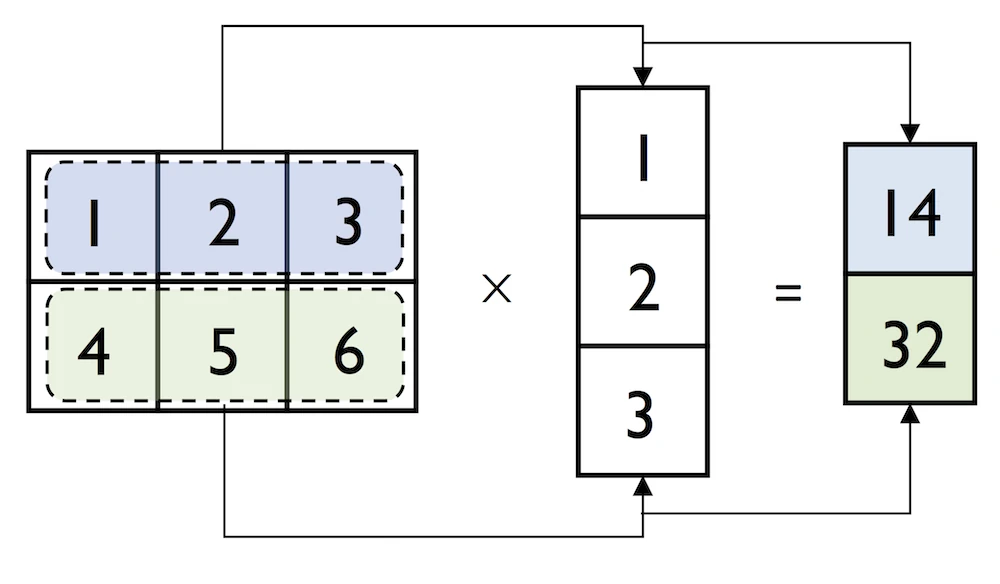
However, if we are working with matrices and vectors, NumPy can be quite forgiving if the dimensions of matrices and one-dimensional arrays do not match exactly -- thanks to broadcasting. The following example yields the same result as the matrix-column vector multiplication, except that it returns a one-dimensional array instead of a two-dimensional one:
然而,如果我们使用矩阵和向量,如果矩阵和一维数组的维数不完全匹配,NumPy可以非常宽容------这要归功于广播。以下示例产生的结果与矩阵列向量乘法相同,只是它返回的是一维数组而不是二维数组:
但是这里,貌似不是因为广播。
一维数组与矩阵乘法:计算规则与内存实现
一、计算规则:一维数组 vs 二维列向量
这个例子里其实没有发生真正的广播 ------它展示的是
np.matmul对一维数组的特殊处理规则。关键区别 :二维列向量
[[1],[2],[3]]的形状是3×1,而一维数组[1,2,3]的形状是(3,)。图解
输入 A (矩阵)          输入 B (一维数组)
形状 (2, 3)            形状 (3,)

┌───┬───┬───┐
│ 1 │ 2 │ 3 │┐
├───┼───┼───┤ │ ×   [ 1 , 2 , 3 ]
│ 4 │ 5 │ 6 │ ┘
└───┴───┴───┘

matmul 规则:右操作数是一维时,
临时把它当成列向量 (3,) → (3,1) 参与运算
      ┌───┐
      │ 1 │
      │ 2 │
      │ 3 │
      └───┘
逐行点乘
第 1 行:  1×1 + 2×2 + 3×3  =  1 + 4 + 9   = 14
第 2 行:  4×1 + 5×2 + 6×3  =  4 + 10 + 18 = 32
输出对比
二维列向量做法              一维数组做法 (本例)
形状 (2, 1)                 形状 (2,)
┌────┐
│ 14 │                      [ 14 , 32 ]
│ 32 │
└────┘
小结 :
np.matmul(matrix, row_vector)里,matmul看到右边是一维数组,就临时把它补成列向量去做矩阵乘法,算完再把补出来的那一维去掉。所以计算过程和二维列向量完全一样,得到[14, 32],但结果是一维数组而不是二维的[[14],[32]]。
二、内存实现
在内存层面,NumPy 数组的核心是一块连续的一维内存 + 一组描述如何解读它的元数据。矩阵乘法本身不移动数据,它靠元数据(shape/strides)去寻址。
1. 数组在内存里的样子
┌─────────────────────────────┐
│  元数据 (header)             │
│    - shape:   (2, 3)         │
│    - strides: (24, 8)        │  ← 每维走一步跳多少字节
│    - dtype:   float64 (8B)   │
│    - data ptr ───────────┐   │
└──────────────────────────┼───┘
                           ↓
┌────┬────┬────┬────┬────┬────┐   连续内存 (row-major / C 序)
│ 1  │ 2  │ 3  │ 4  │ 5  │ 6  │   每格 8 字节
└────┴────┴────┴────┴────┴────┘
  0    8   16   24   32   40   ← 字节偏移
matrix[i][j]的地址 =data_ptr + i*24 + j*8。二维的"行列"只是 strides 制造的视图,底层永远是那条一维带子。2. 一维数组
[1,2,3]在内存里
┌─────────────────────────────┐
│  shape:   (3,)               │
│  strides: (8,)               │
│  data ptr ───────────┐       │
└──────────────────────┼───────┘
                       ↓
┌────┬────┬────┐
│ 1  │ 2  │ 3  │
└────┴────┴────┘
  0    8   16
内存里
[1,2,3]和列向量[[1],[2],[3]]的数据完全一样,区别只在元数据:
一维 (3,)               列向量 (3,1)
shape=(3,)              shape=(3,1)
strides=(8,)            strides=(8,8)
       └── 同一块内存 [1,2,3] ──┘
所以"补成列向量"在内存上不产生拷贝,只是换一副 shape/strides 的眼镜去看同一块数据。
3. matmul 计算时的内存访问
matmul不会生成中间的列向量对象,它直接把两个 data 指针和 strides 交给底层的 BLAS 例程(如 OpenBLAS 的dgemm/dgemv)。计算结果[i] = Σ matrix[i,k] * vec[k]:
vec 指针扫描 →┌──┬──┬──┐ │1 │2 │3 │ └──┴──┴──┘ matrix 指针 ↓ ↓ ↓ ┌──┬──┬──┐ 行0: 1 2 3 点乘 → 14 ─┐ │1 │2 │3 │ (偏移 0,8,16) │ 写入输出 ├──┼──┼──┤ │ 连续内存 │4 │5 │6 │ 行1: 4 5 6 点乘 → 32 ─┤ └──┴──┴──┘ (偏移 24,32,40) ↓ ┌────┬────┐ │ 14 │ 32 │ shape=(2,) └────┴────┘ strides=(8,)关键点:
- 输出形状由 matmul 规则决定。输入是
(2,3) × (3,),右边一维,所以结果去掉那一维,得到(2,)。输出是一块新分配的连续内存,存[14, 32]。- 全程只有输出被分配了新内存,输入数据一次都没拷贝或重排。
- strides 让 BLAS 能按行/列任意步长跳着读,不需要数据物理相邻成"列"。
小结 :NumPy 把"矩阵""向量"这些概念全部落到一块一维连续内存 + shape/strides 元数据上。matmul 处理一维输入时,不实际构造列向量,只是用不同的 strides 解释同一块内存,把指针交给 BLAS 做点乘,最后按维度规则分配一块新内存存放结果
[14,32]。
说明:字节偏移和 strides 基于默认的 C 连续、float64 数组。Fortran 序、切片或转置会导致 strides 不同,但"数据不动、只调整解读方式"的原理一致。BLAS 的具体函数选择(gemv vs gemm)也可能因 NumPy 版本和输入维度而异。
In:
python
np.matmul(matrix, row_vector)Out:
python
array([14, 32])Similarly, we can compute the dot-product between two vectors (here: the vector norm)
同样,我们可以计算两个向量之间的点积(这里:向量范数)
In:
python
np.matmul(row_vector, row_vector)Out:
python
14NumPy has a special dot function that behaves similar to matmul on pairs of one- or two-dimensional arrays -- its underlying implementation is different though, and one or the other can be slightly faster on specific machines and versions of BLAS:
NumPy有一个特殊的点函数,它在一对或二维数组上的行为类似于matmul------但它的底层实现是不同的,在特定的机器和BLAS版本上,其中一个可能会稍微快一些:
In:
python
np.dot(matrix, row_vector)Out:
python
array([14, 32])Note that an even more convenient way for executing np.dot is using the @ symbol with NumPy arrays:
请注意,执行np.dot的一种更方便的方法是在NumPy数组中使用@符号:
In:
python
matrix @ row_vectorOut:
python
array([14, 32])Similar to the examples above we can use matmul or dot to multiply two matrices (here: two-dimensional arrays). In this context, NumPy arrays have a handy transpose method to transpose matrices if necessary:
与上面的例子类似,我们可以使用matmul或dot来乘两个矩阵(这里是二维数组)。在这种情况下,NumPy数组有一个方便的转置方法,可以在必要时转置矩阵:
In:
python
matrix = np.array([[1, 2, 3],
                   [4, 5, 6]])
matrix.transpose()
Out:
python
array([[1, 4],
       [2, 5],
       [3, 6]])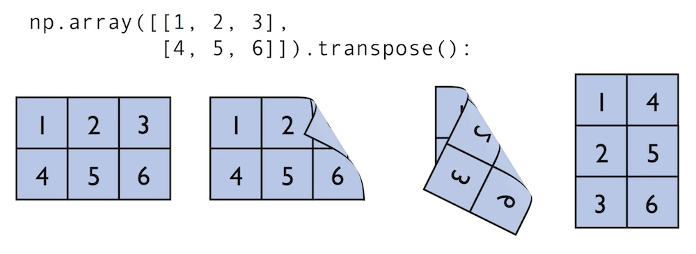
NumPy transpose 的内存实现
核心概念:数据 + strides
numpy 数组由两部分组成:
- 一块连续的内存缓冲区(data buffer),存着实际数值
- 一组元数据 ,最重要的是
shape和strides
strides表示"在每个维度上走一步,内存地址要跳多少字节"。原始数组的内存布局
pythonmatrix = np.array([[1, 2, 3], [4, 5, 6]])假设是
int64(8 字节)。内存里数据是按行连续存放的(C order):
内存地址:   0    8    16   24   32   40
          ┌────┬────┬────┬────┬────┬────┐
数据缓冲:  │ 1  │ 2  │ 3  │ 4  │ 5  │ 6  │
          └────┴────┴────┴────┴────┴────┘
              ↑    ↑    ↑    ↑    ↑    ↑
索引:    (0,0)(0,1)(0,2)(1,0)(1,1)(1,2)
元数据:
shape   = (2, 3)
strides = (24, 8)     # 行跳24字节(3个int64), 列跳8字节
访问
matrix[i][j]的地址计算:
地址 = base + i * strides[0] + j * strides[1]
     = base + i * 24 + j * 8
例:
matrix[1][2]=base + 1*24 + 2*8=base + 40→ 值是6transpose 之后:内存没变,只交换了 strides
pythonmatrix.transpose() # 或 matrix.T关键:数据缓冲区一个字节都没动。 numpy 只是把
shape和strides里的元素倒过来:
内存地址:   0    8    16   24   32   40
          ┌────┬────┬────┬────┬────┬────┐
数据缓冲:  │ 1  │ 2  │ 3  │ 4  │ 5  │ 6  │   ← 完全相同的那块内存
          └────┴────┴────┴────┴────┴────┘
新元数据:
shape   = (3, 2)      # 从 (2,3) 反转
strides = (8, 24)     # 从 (24,8) 反转  ← 只是交换了顺序
转置后的地址公式:
地址 = base + i * strides[0] + j * strides[1]
     = base + i * 8 + j * 24
转置后应为:
T = [[1, 4],
     [2, 5],
     [3, 6]]
验证:
T[0][0]=base + 0 + 0= 地址 0 →1T[0][1]=base + 0 + 24= 地址 24 →4T[1][0]=base + 8 + 0= 地址 8 →2T[2][1]=base + 16 + 24= 地址 40 →6为什么这么设计
- O(1) 时间、零拷贝:转置 1GB 的矩阵和转置 2×3 的矩阵一样快
- 返回的是 view(视图),不是 copy。修改转置结果会影响原数组:
pythonT = matrix.transpose() T[0][0] = 99 print(matrix[0][0]) # 输出 99,因为共享同一块内存代价:内存不再连续
转置后数组变成 F-contiguous(列优先连续) 而非 C-contiguous:
pythonmatrix.flags['C_CONTIGUOUS'] # True matrix.T.flags['C_CONTIGUOUS'] # False matrix.T.flags['F_CONTIGUOUS'] # True有些操作(某些
reshape,或需要连续内存的 C 扩展)会因此触发真正的数据拷贝。强制拿到行连续的新内存:
pythonT_copy = np.ascontiguousarray(matrix.T) # 这次才真的复制数据一句话总结
transpose不搬数据,只是把shape和strides反转,让 numpy 用不同的步长去读同一块内存------所以它是零拷贝的视图操作。
In:
python
np.dot(matrix, matrix.transpose())Out:
python
array([[14, 32],
       [32, 77]])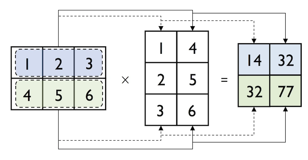
While transpose can be annoyingly verbose for implementing linear algebra operations -- think of PEP8's 80 character per line recommendation -- NumPy has a shorthand for that: T:
虽然转置在实现线性代数操作时可能会非常冗长------想想PEP8的每行80个字符的建议------但NumPy对此有一个简写:T:
In:
python
matrix.TOut:
python
array([[1, 4],
       [2, 5],
       [3, 6]])
While this section demonstrates some of the basic linear algebra operations carried out on NumPy arrays that we use in practice, you can find an additional function in the documentation of NumPy's submodule for linear algebra: numpy.linalg. If you want to perform a particular linear algebra routine that is not implemented in NumPy, it is also worth consulting the scipy.linalg documentation -- SciPy is a library for scientific computing built on top of NumPy.
虽然本节演示了我们在实践中使用的NumPy数组上执行的一些基本线性代数操作,但您可以在NumPy线性代数子模块的文档中找到一个附加函数:NumPy.linalg。如果你想执行NumPy中没有实现的特定线性代数例程,也值得参考scipy.linalg文档------scipy是一个基于NumPy构建的科学计算库。
I want to mention that there is also a special matrix type in NumPy. NumPy matrix objects are analogous to NumPy arrays but are restricted to two dimensions. Also, matrices define certain operations differently than arrays; for instance, the * operator performs matrix multiplication instead of element-wise multiplication. However, NumPy matrix is less popular in the science community compared to the more general array data structure.
我想提到的是,NumPy中还有一种特殊的矩阵类型。NumPy矩阵对象类似于NumPy数组,但仅限于二维。此外,矩阵对某些操作的定义与数组不同;例如,*运算符执行矩阵乘法而不是元素乘法。然而,与更通用的数组数据结构相比,NumPy矩阵在科学界不太受欢迎。
SciPy
SciPy is another open-source library from Python's scientific computing stack. SciPy includes submodules for integration, optimization, and many other kinds of computations that are out of the scope of NumPy itself. We will not cover SciPy as a library here, since it can be more considered as an "add-on" library on top of NumPy.
SciPy是Python科学计算堆栈中的另一个开源库。SciPy包括用于集成、优化和NumPy本身范围之外的许多其他类型计算的子模块。我们在这里不会将SciPy作为一个库来介绍,因为它更可以被视为NumPy之上的"附加"库。
I recommend you to take a look at the SciPy documentation to get a brief overview of the different function that exists within this library: https://docs.scipy.org/doc/scipy/reference/
我建议您查看SciPy文档,以简要了解此库中存在的不同功能:https://docs.scipy.org/doc/scipy/reference/
4.10: Matplotlib
What is Matplotlib?
Lastly, we will briefly cover Matplotlib in this article. Matplotlib is a plotting library for Python created by John D. Hunter in 2003. Unfortunately, John D. Hunter became ill and past away in 2012. However, Matplot is still the most mature plotting library, and is being maintained until this day.
最后,本文将简要介绍Matplotlib。Matplotlib是John D.Hunter于2003年创建的Python绘图库。不幸的是,约翰·D·亨特在2012年生病并去世了。然而,Matplot仍然是最成熟的绘图库,并一直维护到今天。
In general, Matplotlib is a rather "low-level" plotting library, which means that it has a lot of room for customization. The advantage of Matplotlib is that it is so customizable; the disadvantage of Matplotlib is that it is so customizable -- some people find it a little bit too verbose due to all the different options.
一般来说,Matplotlib是一个相当"低级"的绘图库,这意味着它有很大的定制空间。Matplotlib的优点是它是可定制的;Matplotlib的缺点是它是可定制的------有些人觉得它有点过于冗长,因为它有各种不同的选项。
In any case, Matplotlib is among the most widely used plotting library and the go-to choice for many data scientists and machine learning researchers and practictioners.
无论如何,Matplotlib是使用最广泛的绘图库之一,也是许多数据科学家、机器学习研究人员和实践者的首选。
In my opinion, the best way to work with Matplotlib is to use the Matplotlib gallery on the official website at https://matplotlib.org/gallery/index.html often. It contains code examples for creating various different kinds of plots, which are useful as templates for creating your own plots. Also, if you are completely new to Matplotlib, I recommend the tutorials at https://matplotlib.org/tutorials/index.html.
在我看来,使用Matplotlib的最佳方式是使用官方网站上的Matplotlibgalleryhttps://matplotlib.org/gallery/index.html经常。它包含创建各种不同类型绘图的代码示例,这些示例可用作创建自己绘图的模板。此外,如果您是Matplotlib的新手,我建议您使用以下教程https://matplotlib.org/tutorials/index.html .
In this section, we will look at a few very simple examples, which should be very intuitive and shouldn't require much explanation.
在本节中,我们将看一些非常简单的例子,这些例子应该非常直观,不需要太多解释。
In:
python
%matplotlib inline
import matplotlib.pyplot as plt
The main plotting functions of Matplotlib are contained in the pyplot module, which we imported above. Note that the %matplotlib inline command is an "IPython magic" command. This particular %matplotlib inline is specific to Jupyter notebooks (which, in our case, use an IPython kernel) to show the plots "inline," that is, the notebook itself.
Matplotlib的主要绘图功能包含在我们上面导入的pyplot模块中。请注意,%matplotlib内联命令是一个"IPython magic"命令。这个特定的%matplotlib内联是Jupyter笔记本特有的(在我们的例子中,它使用IPython内核),用于"内联"显示绘图,即笔记本本身。
Plotting Functions and Lines
In:
python
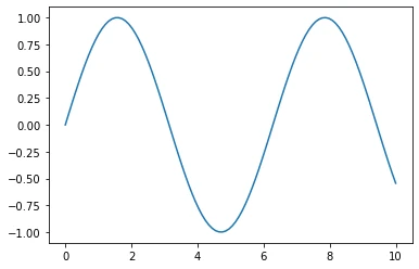
x = np.linspace(0, 10, 100)
plt.plot(x, np.sin(x))
plt.show()
Out:

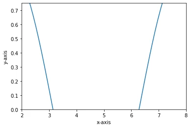
Add axis ranges and labels:添加轴范围和标签:
In:
python
x = np.linspace(0, 10, 100)
plt.plot(x, np.sin(x))
plt.xlim([2, 8])
plt.ylim([0, 0.75])
plt.xlabel('x-axis')
plt.ylabel('y-axis')
plt.show()
Out:
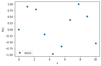
In:
python
x = np.linspace(0, 10, 10)
plt.plot(x, np.sin(x), label=('sin(x)'), linestyle='', marker='o')
plt.ylabel('f(x)')
plt.xlabel('x')
plt.legend(loc='lower left')
plt.show()
Out:
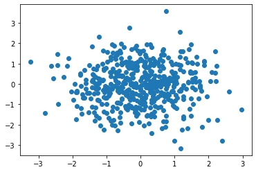
Scatter Plots
In:
python
rng = np.random.RandomState(123)
x = rng.normal(size=500)
y = rng.normal(size=500)
plt.scatter(x, y)
plt.show()
Out:
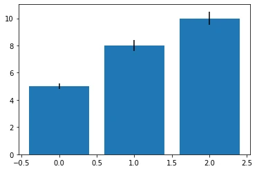
Bar Plots
In:
python
# input data
means = [5, 8, 10]
stddevs = [0.2, 0.4, 0.5]
bar_labels = ['bar 1', 'bar 2', 'bar 3']
# plot bars
x_pos = list(range(len(bar_labels)))
plt.bar(x_pos, means, yerr=stddevs)
plt.show()
Out:
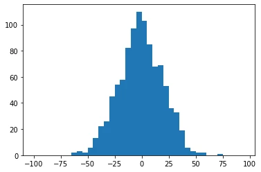
Histograms
In:
python
rng = np.random.RandomState(123)
x = rng.normal(0, 20, 1000)
# fixed bin size
bins = np.arange(-100, 100, 5) # fixed bin size
plt.hist(x, bins=bins)
plt.show()
Out:
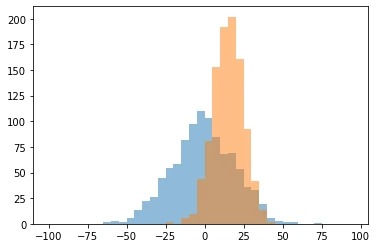
In:
python
rng = np.random.RandomState(123)
x1 = rng.normal(0, 20, 1000)
x2 = rng.normal(15, 10, 1000)
# fixed bin size
bins = np.arange(-100, 100, 5) # fixed bin size
plt.hist(x1, bins=bins, alpha=0.5)
plt.hist(x2, bins=bins, alpha=0.5)
plt.show()
Out:
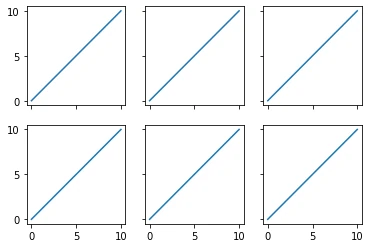
Subplots
In:
python
x = range(11)
y = range(11)
fig, ax = plt.subplots(nrows=2, ncols=3,
                       sharex=True, sharey=True)
for row in ax:
    for col in row:
        col.plot(x, y)
plt.show()
Out:
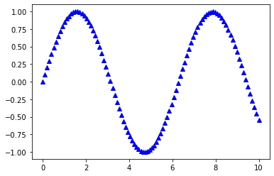
Colors and Markers
In:
python
x = np.linspace(0, 10, 100)
plt.plot(x, np.sin(x),
         color='blue',
         marker='^',
         linestyle='')
plt.show()
Out:
Saving Plots
The file format for saving plots can be conveniently specified via the file suffix (.eps, .svg, .jpg, .png, .pdf, .tiff, etc.). Personally, I recommend using a vector graphics format (.eps, .svg, .pdf) whenever you can, which usually results in smaller file sizes than bitmap graphics (.jpg, .png, .bmp, tiff) and does not have a limited resolution.
保存绘图的文件格式可以通过文件后缀(.eps、.svg、.jpg、.png、.pdf、.tiff等)方便地指定。就个人而言,我建议尽可能使用矢量图形格式(.eps、.svg、.pdf),这通常会导致比位图图形(.jpg、.png、.bmp、tiff)更小的文件大小,并且没有有限的分辨率。
In:
python
x = np.linspace(0, 10, 100)
plt.plot(x, np.sin(x))
plt.savefig('myplot.png', dpi=300)
plt.savefig('myplot.pdf')
plt.show()
Out: