接续上一篇笔记:扩散模型初探(一)。
这里主要探讨一下NCSN与DDPM。我看了一下论文研究时间,相差不久,作者都是尝试从去噪的角度去做的,过程看似不同,但最后数学上居然能统一起来。两者殊途同归,真是妙啊。。
NCSN的介绍
NCSN 简介
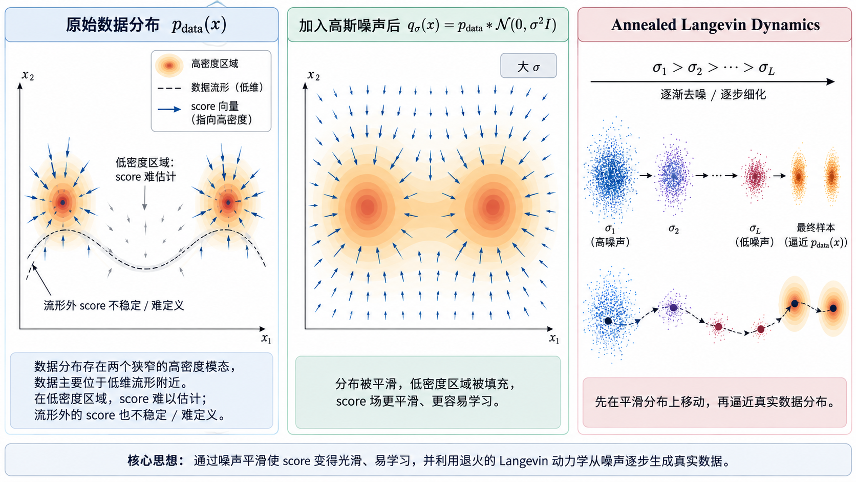
NCSN(Noise Conditional Score Network)的核心思想是:
给真实数据加入不同强度的高斯噪声, x ~ = x + σ z , z ∼ N ( 0 , I ) , \tilde{x}=x+\sigma z,\quad z\sim\mathcal{N}(0,I), x~=x+σz,z∼N(0,I), 然后训练网络 s θ ( x ~ , σ ) s_\theta(\tilde{x},\sigma) sθ(x~,σ),去逼近加噪分布的 score:
s θ ( x ~ , σ ) ≈ ∇ x ~ log q σ ( x ~ ) . s_\theta(\tilde{x},\sigma)\approx \nabla_{\tilde{x}}\log q_\sigma(\tilde{x}). sθ(x~,σ)≈∇x~logqσ(x~).
论文使用多个噪声尺度 σ 1 > σ 2 > ⋯ > σ L , \sigma_1>\sigma_2>\cdots>\sigma_L, σ1>σ2>⋯>σL, 让同一个网络同时学习不同噪声水平下的数据分布。
Loss 推导
训练采用 Denoising Score Matching。由于 q σ ( x ~ ∣ x ) = N ( x , σ 2 I ) , q_\sigma(\tilde{x}\mid x)=\mathcal{N}(x,\sigma^2I), qσ(x~∣x)=N(x,σ2I), 因此有
∇ x ~ log q σ ( x ~ ∣ x ) = − x ~ − x σ 2 . \nabla_{\tilde{x}}\log q_\sigma(\tilde{x}\mid x) =-\frac{\tilde{x}-x}{\sigma^2}. ∇x~logqσ(x~∣x)=−σ2x~−x. 于是训练 loss 可以写成
ℓ ( θ ; σ ) = 1 2 E ∥ s θ ( x \~ , σ ) + x \~ − x σ 2 ∥ 2 \boxed{ \ell(\theta;\sigma) =\frac12 \mathbb{E} \left \\left\\\| s_\\theta(\\tilde{x},\\sigma) + \\frac{\\tilde{x}-x}{\\sigma\^2} \\right\\\|\^2 \\right } ℓ(θ;σ)=21E sθ(x\~,σ)+σ2x\~−x 2
又因为 x ~ = x + σ z , \tilde{x}=x+\sigma z, x~=x+σz, 所以 x ~ − x σ 2 = z σ , \frac{\tilde{x}-x}{\sigma^2} =\frac{z}{\sigma}, σ2x~−x=σz, 从而有
s θ ( x + σ z , σ ) ≈ − z σ . s_\theta(x+\sigma z,\sigma) \approx -\frac{z}{\sigma}. sθ(x+σz,σ)≈−σz. 也就是说,本质上是给网络一个加噪样本,让它学习指向高概率区域的方向。
多个噪声尺度下的总 loss 为 L ( θ ) = 1 L ∑ i = 1 L λ ( σ i ) ℓ ( θ ; σ i ) , L(\theta) =\frac1L \sum_{i=1}^{L} \lambda(\sigma_i)\ell(\theta;\sigma_i), L(θ)=L1i=1∑Lλ(σi)ℓ(θ;σi), 论文中取 λ ( σ ) = σ 2 \lambda(\sigma)=\sigma^2 λ(σ)=σ2 来平衡不同噪声尺度的 loss。
Annealed Langevin Dynamics (退火郎之万动力学)
训练完成后,使用 Annealed Langevin Dynamics 进行生成。
首先从随机噪声初始化 x 0 ∼ π ( x ) , x_0\sim \pi(x), x0∼π(x), 然后按照 σ 1 > σ 2 > ⋯ > σ L \sigma_1>\sigma_2>\cdots>\sigma_L σ1>σ2>⋯>σL 逐渐降低噪声水平。在第 i i i 个噪声尺度下,重复执行 x t = x t − 1 + α i 2 s θ ( x t − 1 , σ i ) + α i z t , z t ∼ N ( 0 , I ) , x_t= x_{t-1} + \frac{\alpha_i}{2} s_\theta(x_{t-1},\sigma_i) + \sqrt{\alpha_i}z_t, \qquad z_t\sim\mathcal N(0,I), xt=xt−1+2αisθ(xt−1,σi)+αi zt,zt∼N(0,I),其中步长为 α i = ϵ σ i 2 σ L 2 . \alpha_i=\epsilon\frac{\sigma_i^2}{\sigma_L^2}. αi=ϵσL2σi2.
每个噪声尺度运行若干步 Langevin dynamics,并将当前阶段的最终样本作为下一个更小噪声尺度的初始值: q σ 1 → q σ 2 → ⋯ → q σ L ≈ p data . q_{\sigma_1} \rightarrow q_{\sigma_2} \rightarrow \cdots \rightarrow q_{\sigma_L} \approx p_{\text{data}}. qσ1→qσ2→⋯→qσL≈pdata.直观上,大噪声阶段负责全局探索,小噪声阶段负责逐步细化,
最终从随机噪声生成接近真实数据分布的样本。 DSM 负责训练 score , Annealed Langevin 负责生成 \boxed{ \text{DSM 负责训练 score}, \text{Annealed Langevin 负责生成} } DSM 负责训练 score,Annealed Langevin 负责生成
NCSN 与 DDPM 的联系
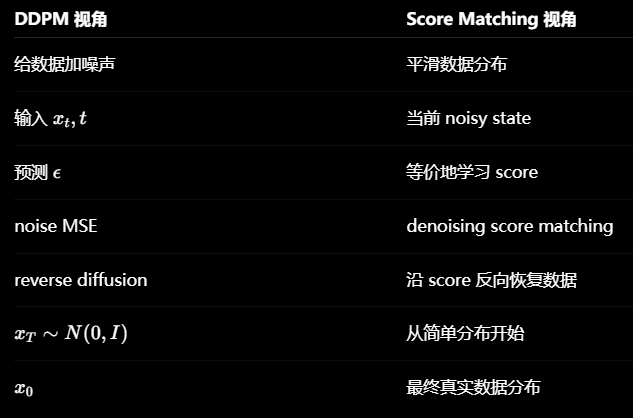
NCSN 和 DDPM 的核心联系是:两者都在学习不同噪声水平下的数据结构,本质上可以通过 score 联系起来。
对于 DDPM,有
∇ x t log q ( x t ∣ x 0 ) = − ϵ 1 − α ˉ t . \nabla_{x_t}\log q(x_t|x_0) =-\frac{\epsilon}{\sqrt{1-\bar{\alpha}_t}}. ∇xtlogq(xt∣x0)=−1−αˉt ϵ.
因此噪声预测网络和 score 网络之间可以建立对应关系:
s θ ( x t , t ) = − ϵ θ ( x t , t ) 1 − α ˉ t \boxed{ s_\theta(x_t,t) =-\frac{\epsilon_\theta(x_t,t)} {\sqrt{1-\bar{\alpha}_t}} } sθ(xt,t)=−1−αˉt ϵθ(xt,t)
所以:
DDPM 的 Noise Prediction ⟺ NCSN 的 Score Prediction \boxed{ \text{DDPM 的 Noise Prediction} \Longleftrightarrow \text{NCSN 的 Score Prediction} } DDPM 的 Noise Prediction⟺NCSN 的 Score Prediction
主要区别
- NCSN:在每个噪声尺度下运行多步 Langevin Dynamics,再逐渐降低噪声。
- DDPM :定义离散的 reverse diffusion chain,按照 x T → x T − 1 → ⋯ → x 0 x_T \rightarrow x_{T-1} \rightarrow \cdots \rightarrow x_0 xT→xT−1→⋯→x0 逐步去噪。
从后来的统一视角来看,NCSN 和 DDPM 可以看作 score-based / diffusion generative modeling 的两种不同表述。
NCSN 简单复现
这个实例实现的是一个二维 Denoising Score Matching(DSM)生成模型。它不用直接学习数据分布 p ( x ) p(x) p(x),而是学习不同噪声尺度下的 score,即当前一个点在二维空间的某个位置时,应该往哪个方向移动,才能进入更高概率的数据区域。实验可以分成以下 5 个阶段:
-
构造真实数据分布
使用 8 个二维 Gaussian cluster,均匀分布在圆环上 -
给真实数据加入不同强度的高斯噪声 。从真实样本 x 0 x_0 x0 出发:
x ~ = x 0 + σ ϵ , ϵ ∼ N ( 0 , I ) \tilde{x}=x_0+\sigma\epsilon, \epsilon\sim\mathcal N(0,I) x~=x0+σϵ,ϵ∼N(0,I) 其中 σ \sigma σ 控制噪声大小。代码会随机选择不同的 σ \sigma σ ,让网络同时学习多个噪声尺度。 -
训练 Score Network :由于我们自己知道加入了什么噪声,因此可以直接构造目标 score。训练过程可以概括成:
python真实数据 x0 ↓ 随机采样 sigma ↓ 加 Gaussian noise ↓ 得到 noisy sample ↓ ScoreNet ↓ 预测 score ↓ 与真实 score 做 MSE -
可视化学到的 Score Field:训练后,在二维平面上放很多网格点,让模型预测每个位置的 score。
-
利用 Score 生成新样本 :最后从随机点开始,通过 Annealed Langevin Dynamics。
python随机噪声点 ↓ 高 sigma score 引导大方向 ↓ 中 sigma 调整结构 ↓ 小 sigma 精细收敛 ↓ 8 个 Gaussian cluster
实现代码如下:
python
import math
import os

import numpy as np
import torch
import torch.nn as nn
import torch.nn.functional as F

import matplotlib.pyplot as plt


# ============================================================
# Config
# ============================================================

DEVICE = "cuda" if torch.cuda.is_available() else "cpu"

TRAIN_STEPS = 5000
BATCH_SIZE = 1024
LR = 1e-3

OUTPUT_DIR = "./score_matching_results"

os.makedirs(
    OUTPUT_DIR,
    exist_ok=True
)

print("device:", DEVICE)


# ============================================================
# 1. 真实数据分布
#
# 8 个 Gaussian 分布在圆环上
# ============================================================

def sample_data(batch_size):

    num_modes = 8

    radius = 2.0

    angles = torch.arange(
        num_modes,
        device=DEVICE
    ) * (
        2 * math.pi / num_modes
    )

    centers = torch.stack([
        radius * torch.cos(angles),
        radius * torch.sin(angles)
    ], dim=1)

    # 随机选择一个 Gaussian mode
    labels = torch.randint(
        0,
        num_modes,
        (batch_size,),
        device=DEVICE
    )

    center = centers[labels]

    # 每个 mode 自身也有一点 variance
    x = center + 0.08 * torch.randn(
        batch_size,
        2,
        device=DEVICE
    )

    return x


# ============================================================
# 2. Score Network
#
# 输入:
#
# x_sigma : [x1, x2]
# sigma
#
# 输出:
#
# score vector:
# [dx1, dx2]
# ============================================================

class ScoreNet(nn.Module):

    def __init__(self):

        super().__init__()

        self.net = nn.Sequential(

            nn.Linear(3, 128),
            nn.SiLU(),

            nn.Linear(128, 128),
            nn.SiLU(),

            nn.Linear(128, 128),
            nn.SiLU(),

            nn.Linear(128, 2)
        )

    def forward(
        self,
        x,
        sigma
    ):

        # 使用 log sigma
        log_sigma = torch.log(
            sigma
        )

        inp = torch.cat([
            x,
            log_sigma
        ], dim=1)

        return self.net(inp)


# ============================================================
# 3. Noise Level
#
# 类似 diffusion 里的不同 timestep
#
# 这里直接使用不同 sigma
# ============================================================

SIGMA_MIN = 0.05
SIGMA_MAX = 1.0


def sample_sigma(batch_size):

    # log-uniform sampling

    log_min = math.log(
        SIGMA_MIN
    )

    log_max = math.log(
        SIGMA_MAX
    )

    u = torch.rand(
        batch_size,
        1,
        device=DEVICE
    )

    log_sigma = (
        log_min
        +
        u * (
            log_max
            -
            log_min
        )
    )

    sigma = torch.exp(
        log_sigma
    )

    return sigma


# ============================================================
# 4. 初始化模型
# ============================================================

model = ScoreNet().to(
    DEVICE
)

optimizer = torch.optim.Adam(
    model.parameters(),
    lr=LR
)


# ============================================================
# 5. Denoising Score Matching
#
#
# noisy_x =
# x0 + sigma * epsilon
#
#
# true score:
#
# -(noisy_x - x0) / sigma^2
#
# =
#
# -epsilon / sigma
#
# ============================================================

loss_history = []

for step in range(
    TRAIN_STEPS
):

    # ----------------------------
    # 1. sample real data
    # ----------------------------

    x0 = sample_data(
        BATCH_SIZE
    )

    # ----------------------------
    # 2. sample noise level
    # ----------------------------

    sigma = sample_sigma(
        BATCH_SIZE
    )

    # ----------------------------
    # 3. Gaussian noise
    # ----------------------------

    epsilon = torch.randn_like(
        x0
    )

    # ----------------------------
    # 4. noisy sample
    # ----------------------------

    noisy_x = (
        x0
        +
        sigma * epsilon
    )

    # ----------------------------
    # 5. true score
    #
    # ∇ log q(noisy_x | x0)
    # ----------------------------

    target_score = (
        -epsilon
        /
        sigma
    )

    # ----------------------------
    # 6. predicted score
    # ----------------------------

    pred_score = model(
        noisy_x,
        sigma
    )

    # ----------------------------
    # 7. DSM loss
    #
    # sigma^2 weighting
    # 避免小 sigma 主导 loss
    # ----------------------------

    loss_per_sample = (
        (
            pred_score
            -
            target_score
        ) ** 2
    ).sum(dim=1)

    weight = (
        sigma[:, 0] ** 2
    )

    loss = (
        weight
        *
        loss_per_sample
    ).mean()

    # ----------------------------
    # optimization
    # ----------------------------

    optimizer.zero_grad()

    loss.backward()

    optimizer.step()

    loss_history.append(
        loss.item()
    )

    if step % 200 == 0:

        print(
            f"step={step:5d} "
            f"loss={loss.item():.6f}"
        )


# ============================================================
# 6. 保存模型
# ============================================================

torch.save(
    model.state_dict(),
    os.path.join(
        OUTPUT_DIR,
        "score_model.pt"
    )
)


# ============================================================
# 7. Loss Curve
# ============================================================

plt.figure(
    figsize=(8, 5)
)

plt.plot(
    loss_history
)

plt.xlabel(
    "Training Step"
)

plt.ylabel(
    "DSM Loss"
)

plt.title(
    "Denoising Score Matching Loss"
)

plt.grid(
    alpha=0.3
)

plt.tight_layout()

plt.savefig(
    os.path.join(
        OUTPUT_DIR,
        "loss_curve.png"
    ),
    dpi=160
)

plt.close()


# ============================================================
# 8. Score Field Visualization
#
# 看模型在每个位置预测:
#
# "往哪里走概率会更高"
# ============================================================

@torch.no_grad()
def plot_score_field(
    sigma_value
):

    model.eval()

    grid_size = 30

    x_range = torch.linspace(
        -4,
        4,
        grid_size
    )

    y_range = torch.linspace(
        -4,
        4,
        grid_size
    )

    xx, yy = torch.meshgrid(
        x_range,
        y_range,
        indexing="xy"
    )

    points = torch.stack([
        xx.reshape(-1),
        yy.reshape(-1)
    ], dim=1).to(
        DEVICE
    )

    sigma = torch.full(
        (
            points.shape[0],
            1
        ),
        sigma_value,
        device=DEVICE
    )

    score = model(
        points,
        sigma
    )

    points = points.cpu()
    score = score.cpu()

    # 防止箭头太长
    norm = torch.norm(
        score,
        dim=1,
        keepdim=True
    )

    score = (
        score
        /
        (
            norm + 1e-6
        )
    )

    real_samples = (
        sample_data(
            3000
        )
        .cpu()
    )

    plt.figure(
        figsize=(7, 7)
    )

    plt.scatter(
        real_samples[:, 0],
        real_samples[:, 1],
        s=5,
        alpha=0.25
    )

    plt.quiver(
        points[:, 0],
        points[:, 1],
        score[:, 0],
        score[:, 1]
    )

    plt.xlim(
        -4,
        4
    )

    plt.ylim(
        -4,
        4
    )

    plt.title(
        f"Learned Score Field sigma={sigma_value}"
    )

    plt.xlabel(
        "x1"
    )

    plt.ylabel(
        "x2"
    )

    plt.grid(
        alpha=0.2
    )

    plt.tight_layout()

    plt.savefig(
        os.path.join(
            OUTPUT_DIR,
            f"score_field_sigma_{sigma_value}.png"
        ),
        dpi=160
    )

    plt.close()


plot_score_field(
    0.1
)

plot_score_field(
    0.3
)

plot_score_field(
    0.8
)


# ============================================================
# 9. Annealed Langevin Dynamics
#
# 根据 score 生成新样本
#
#
# x <- x
#      + step * score(x)
#      + sqrt(2*step) * noise
#
# ============================================================

@torch.no_grad()
def sample_with_langevin(
    num_samples=3000
):

    model.eval()

    # 从简单 Gaussian 开始
    x = 3.0 * torch.randn(
        num_samples,
        2,
        device=DEVICE
    )

    # 从高 noise level
    # 一直走到低 noise level

    sigmas = torch.exp(
        torch.linspace(
            math.log(SIGMA_MAX),
            math.log(SIGMA_MIN),
            20,
            device=DEVICE
        )
    )

    base_step = 1e-4

    for sigma_value in sigmas:

        sigma = torch.full(
            (
                num_samples,
                1
            ),
            sigma_value,
            device=DEVICE
        )

        # 高 sigma 使用更大的 step
        step_size = (
            base_step
            *
            (
                sigma_value
                /
                SIGMA_MIN
            ) ** 2
        )

        for _ in range(
            100
        ):

            score = model(
                x,
                sigma
            )

            noise = torch.randn_like(
                x
            )

            x = (
                x
                +
                step_size
                *
                score
                +
                torch.sqrt(
                    2.0
                    *
                    step_size
                )
                *
                noise
            )

    return x


generated = (
    sample_with_langevin(
        3000
    )
    .cpu()
)

real = (
    sample_data(
        3000
    )
    .cpu()
)


# ============================================================
# 10. Compare Real vs Generated
# ============================================================

plt.figure(
    figsize=(10, 5)
)

plt.subplot(
    1,
    2,
    1
)

plt.scatter(
    real[:, 0],
    real[:, 1],
    s=5,
    alpha=0.5
)

plt.title(
    "Real Data"
)

plt.xlim(
    -4,
    4
)

plt.ylim(
    -4,
    4
)

plt.grid(
    alpha=0.2
)


plt.subplot(
    1,
    2,
    2
)

plt.scatter(
    generated[:, 0],
    generated[:, 1],
    s=5,
    alpha=0.5
)

plt.title(
    "Generated Samples"
)

plt.xlim(
    -4,
    4
)

plt.ylim(
    -4,
    4
)

plt.grid(
    alpha=0.2
)


plt.tight_layout()

plt.savefig(
    os.path.join(
        OUTPUT_DIR,
        "real_vs_generated.png"
    ),
    dpi=160
)

plt.close()


print()
print(
    "Finished."
)

print(
    "Results saved to:",
    OUTPUT_DIR
)
实验结果如下:
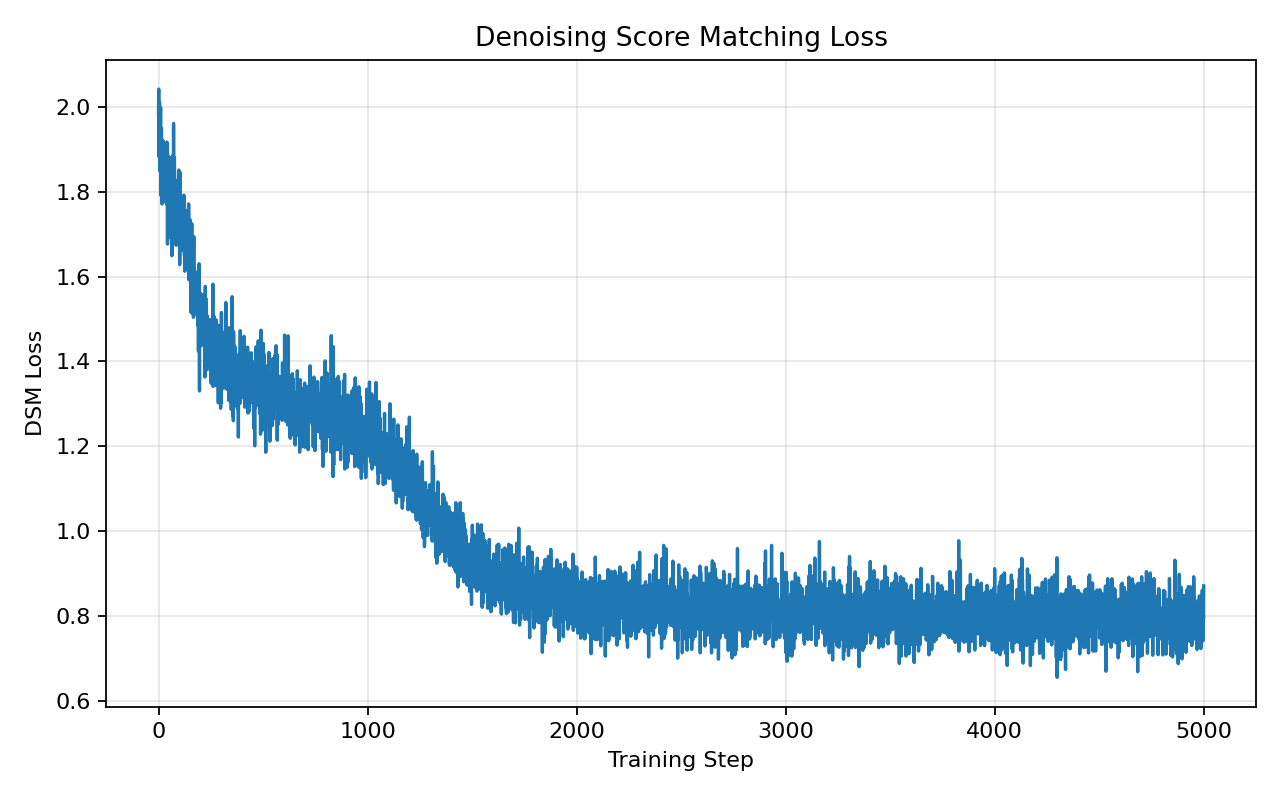
DSM loss 从大约 2.0 很快下降,在 1500~2000 step 左右降到 0.8~0.9,之后基本在这个区间随机波动。这里不要期待 loss 一定接近 0。训练目标是 − ϵ σ -\frac{\epsilon}{\sigma} −σϵ,而网络实际只能根据 ( x ~ , σ ) (\tilde{x}, \sigma) (x~,σ) 来预测它, 对于同一个 noisy point x ~ \tilde x x~,可能存在多个不同的 x 0 , ϵ x_0,\epsilon x0,ϵ 组合,所以目标本身存在条件随机性。DSM 最终学习的是它们的条件期望,对应 noisy marginal distribution 的 score。因此即使模型已经学得很好,训练 loss 也不一定趋近于 0。
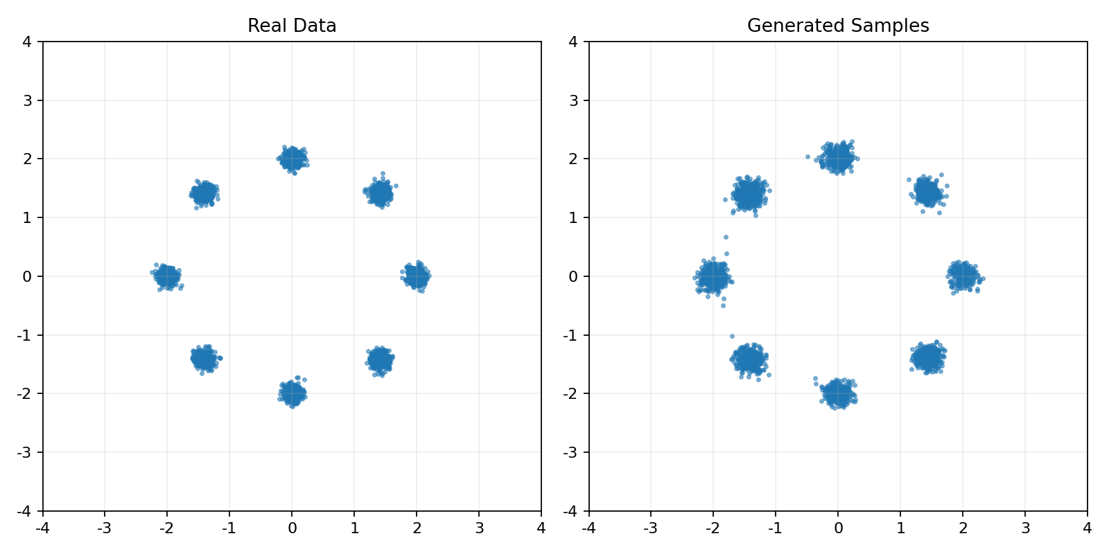
ScoreNet 学到的 vector field 足以把随机初始化的点引导到真实数据的高概率区域。不过生成样本比真实样本稍微"散"一点,而且能看到少数 outlier / mode 之间的点。
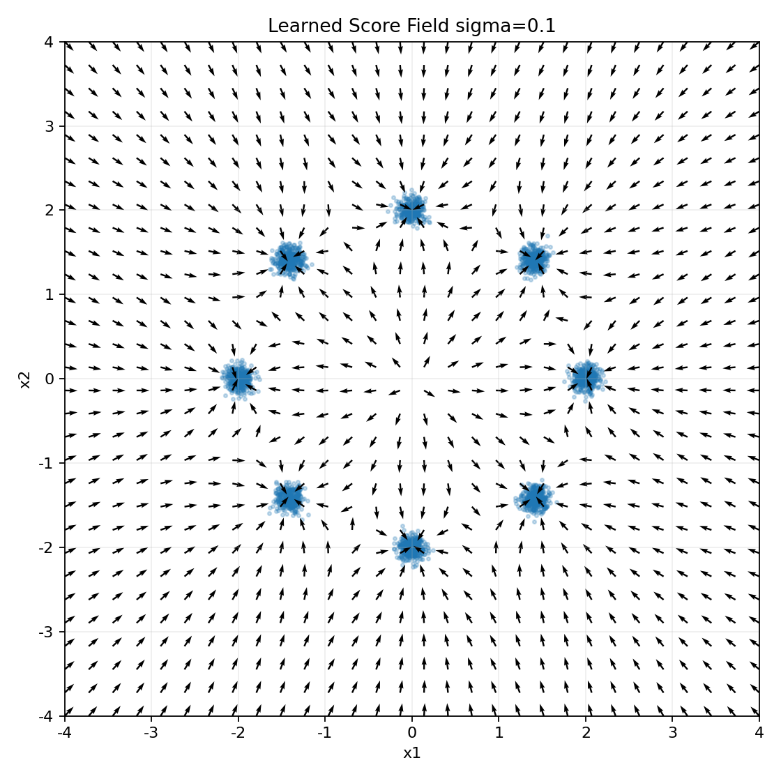
这是低噪声情况。数据分布和真实 8-Gaussian 非常接近。
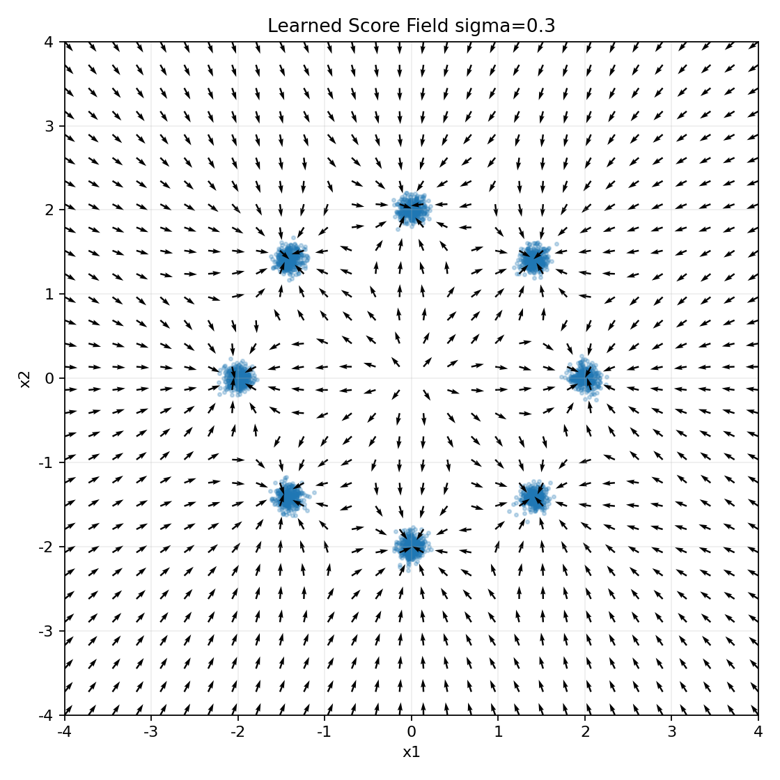
此时数据经过更多 Gaussian smoothing。各个 mode 仍然明显存在,但它们之间开始有一些相互影响。
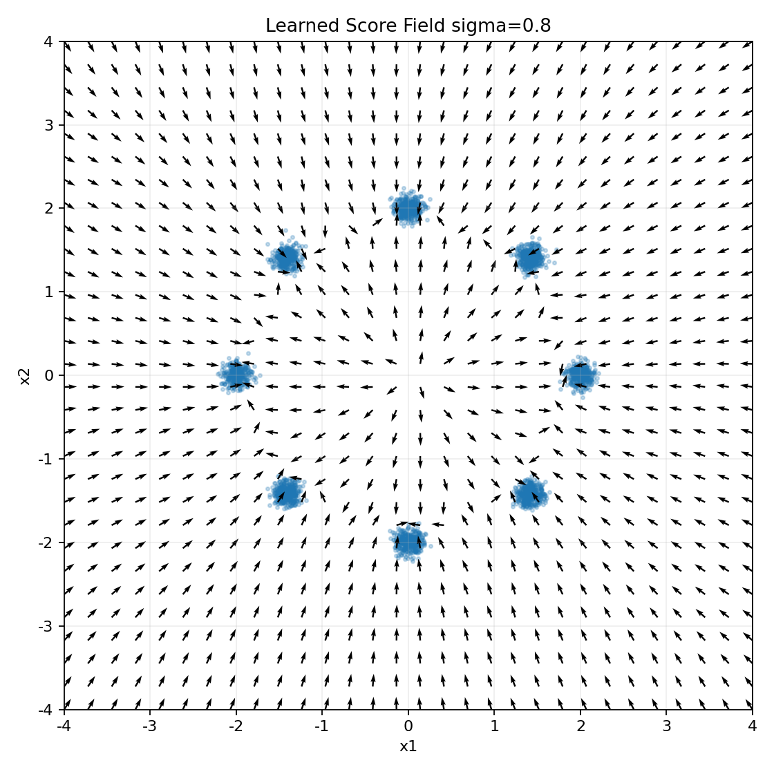
8 个独立 cluster 在 noisy distribution 中已经被明显平滑。
以上仅供参考。