KinectFusion

1.KinectFusion

笔记来源：

论文地址：KinectFusion: Real-time 3D Reconstruction and Interaction Using a Moving Depth Camera*

项目地址：github/KinectFusion

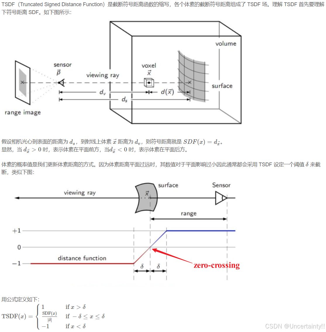
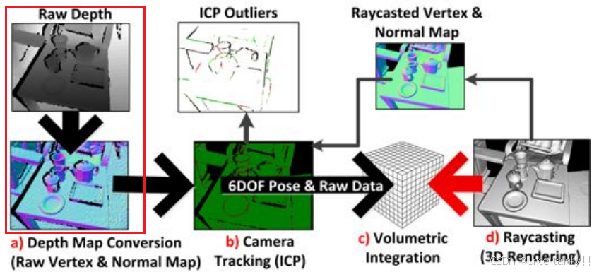
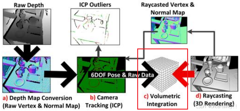
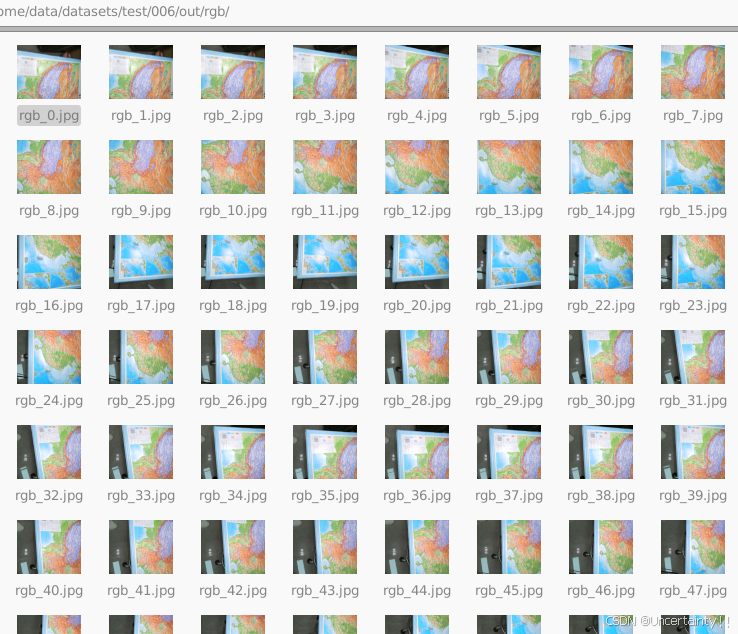
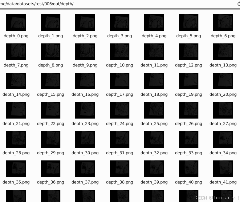
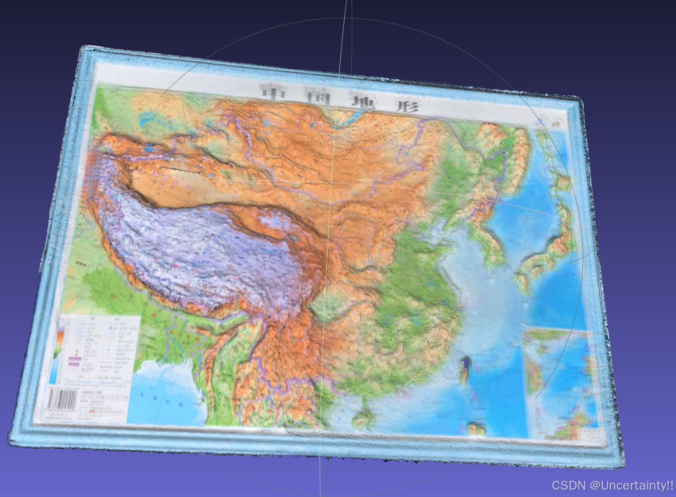
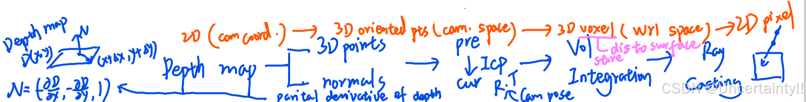
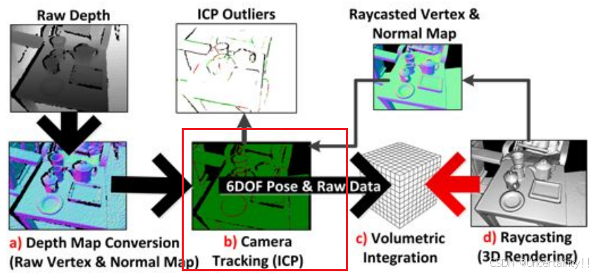
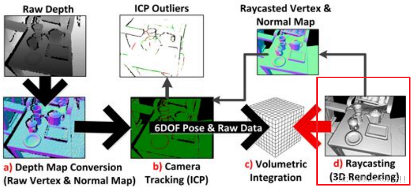
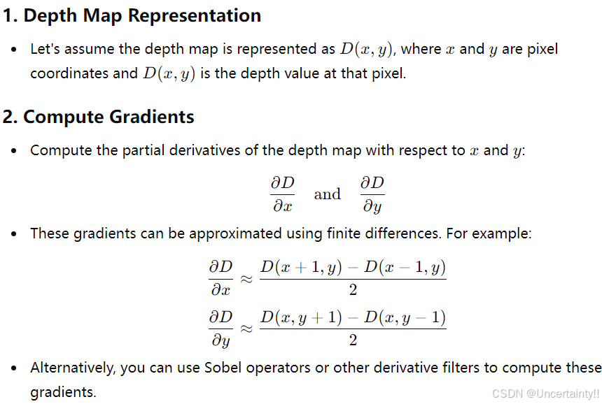
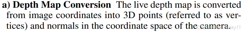
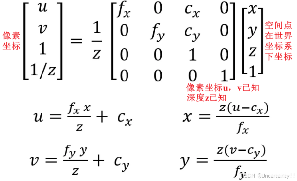
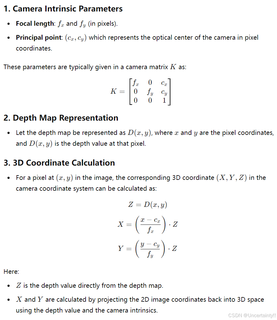
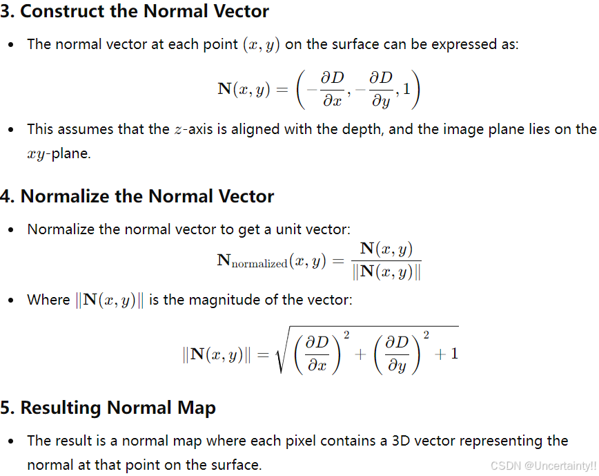
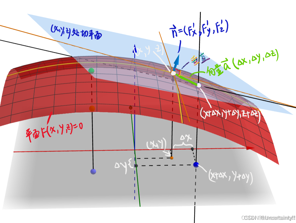
1\] [截断符号距离 \| TSDF, Truncated Signed Distance Function](http://liuxiao.org/kb/3dvision/3d-reconstruction/tsdf-truncated-signed-distance-function/) 本篇对KinectFusion处理流程进行简要了解 KinectFusion功能：使用深度图进行实时三维重建    大致流程： 创建体素网格，第一帧相机在世界坐标系，根据第一帧的 ### 1.1 Depth Map Conversion   从深度图中计算3D坐标点   从深度图中计算法向量   为什么偏导就是点的法向量？ 这个问题在笔者之前的博客中有介绍，[为什么曲面函数的偏导数可以表示其曲面的法向量？](https://aerobaticswu.blog.csdn.net/article/details/133180674)  通过内参矩阵的逆将相机像素平面二维点转到相机空间三维点 pixel： u = （ x , y ） depth： D i ( u ) 3D vertex in camera's coordinate space： v i ( u ) = D i ( u ) K − 1 \[ u , 1 \] ，This results in a single vertex map V i \\text{pixel：}\\bold{u}=（x,y）\\\\ \~\\\\ \\text{depth：}D_i(\\bold{u})\\\\ \~\\\\ \\text{3D vertex in camera's coordinate space：} \\text{v}_i(\\bold{u})=D_i(\\bold{u})K\^{-1}\[\\bold{u},1\]，\\text{This results in a single vertex map} \\text{V}_i\\\\ pixel：u=（x,y） depth：Di(u) 3D vertex in camera's coordinate space：vi(u)=Di(u)K−1\[u,1\]，This results in a single vertex mapVi 相机空间中每个顶点的法向量 normal vectors for each vertex： n i ( u ) = ( v i ( x + 1 , y ) − v i ( x , y ) ) × ( v i ( x , y + 1 ) − v i ( x , y ) ) ，This results in a single vertex map N i \~\\\\ \\text{normal vectors for each vertex：}\\bold{n}_i(\\bold{u})=( \\text{v}_i(x+1,y)-\\text{v}_i(x,y))×(\\text{v}_i(x,y+1)-\\text{v}_i(x,y))，\\text{This results in a single vertex map} \\text{N}_i\\\\ normal vectors for each vertex：ni(u)=(vi(x+1,y)−vi(x,y))×(vi(x,y+1)−vi(x,y))，This results in a single vertex mapNi 通过外参矩阵或旋转矩阵将相机空间中的顶点和每个顶点的法向量转到世界坐标系下 camera pose at time i ： T i = \[ R i ∣ t i \] vertex and normal can be converted into global coordinates： v i g ( u ) = T i v i ( u ) 、 n i g ( u ) = R i n i ( u ) \\text{camera pose at time}\\ i：\\bold{T}_i=\[\\bold{R}_i\|\\bold{t}_i\]\\\\ \~\\\\ \\text{vertex and normal can be converted into global coordinates：}\\bold{v}_i\^g(\\bold{u})=\\bold{T}_i\\bold{v}_i(\\bold{u})、\\bold{n}_i\^g(\\bold{u})=\\bold{R}_i\\bold{n}_i(\\bold{u}) camera pose at time i：Ti=\[Ri∣ti\] vertex and normal can be converted into global coordinates：vig(u)=Tivi(u)、nig(u)=Rini(u) ### 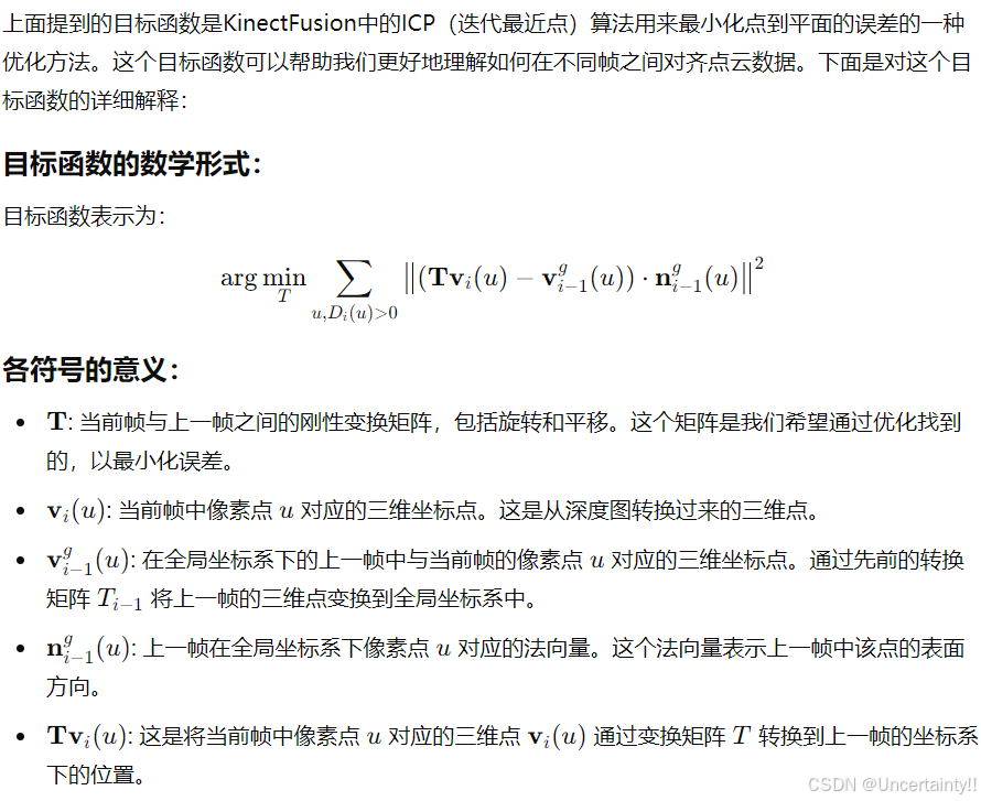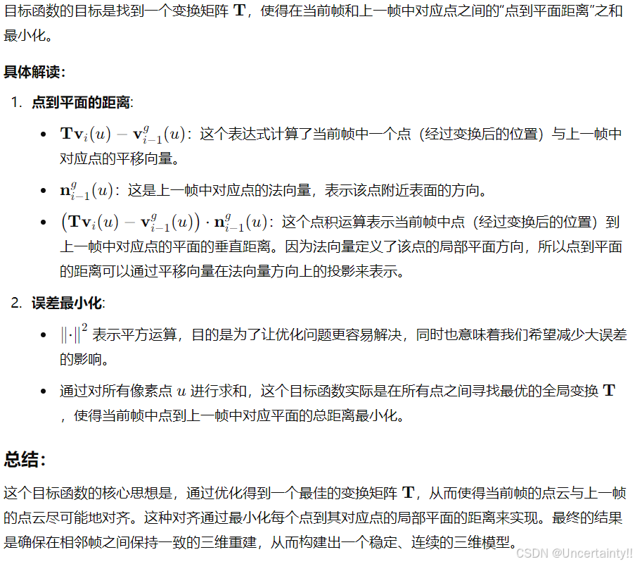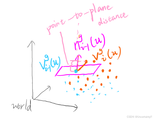1.2 Camera Tracking   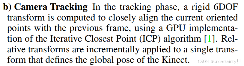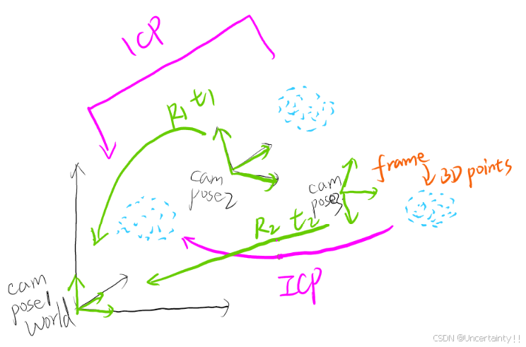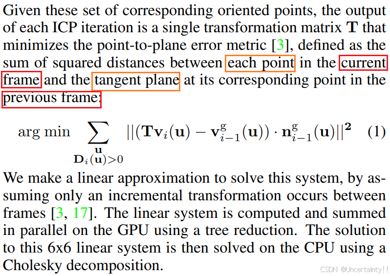该步骤生成的3D点用作ICP求解位姿R，t 第一帧时相机坐标系在世界坐标系的原点，相机平面像素点由内参矩阵得到一组3D点，第二帧也由内参矩阵得到一组3D点，这两组3D点进行ICP得到第二帧到世界坐标系的旋转矩阵 R 1 R_1 R1和平移向量 t 1 t_1 t1，后续帧重复这个操作（第n帧包含了前n-1帧的所有点，依次累积）最终世界坐标系中就会有融合各个帧得到的一组点云  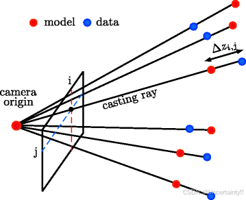两组点云ICP的第一步需要找到两组点云之间的匹配点（或者说是重合的部分） 两组点云依靠这个重合部分进行融合  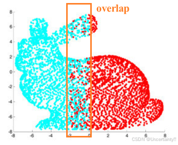两组点云依靠重合部分进行融合  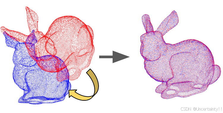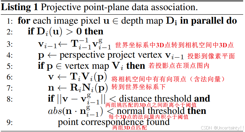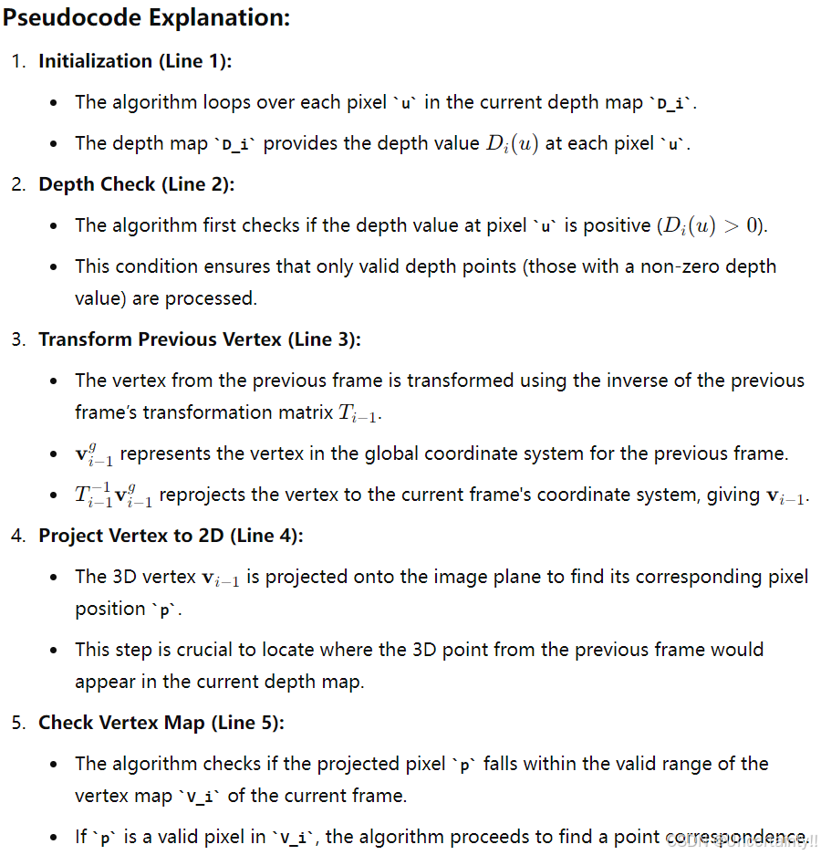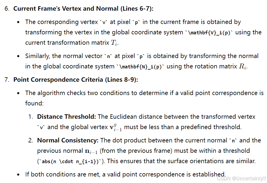文章中用于点云匹配的算法 将前一帧的点（包含前面所有点）投影到当前帧的目的是寻找前一帧和当前帧的匹配点，通过匹配点ICP得以求解获得位姿        ### 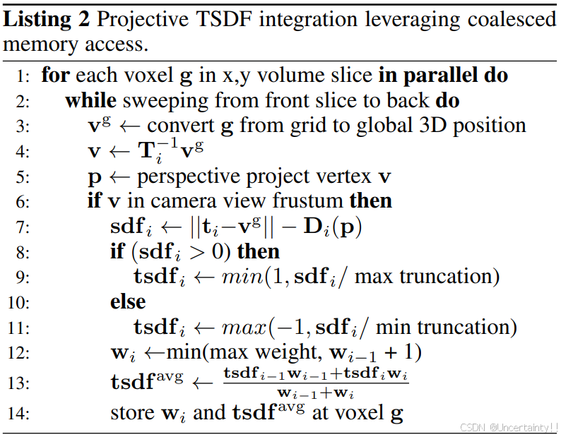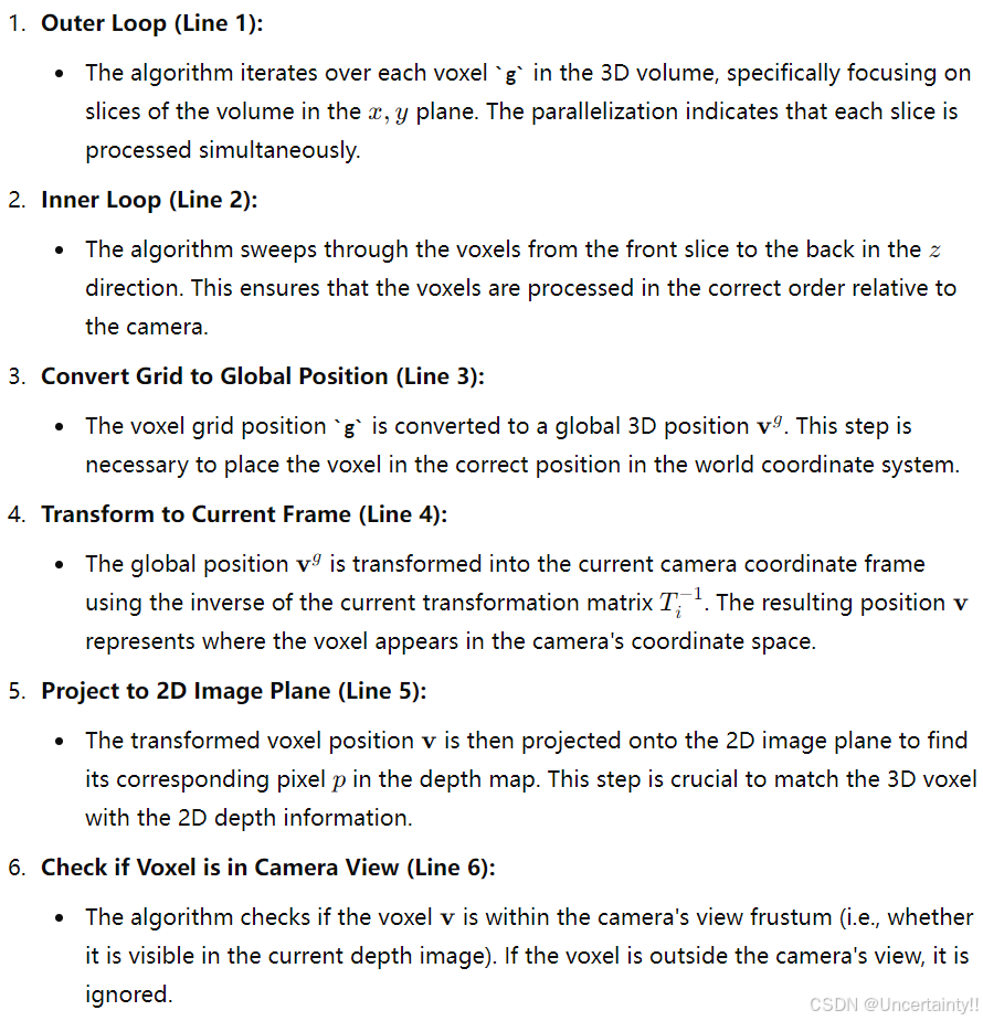1.3 Volumetric Integration 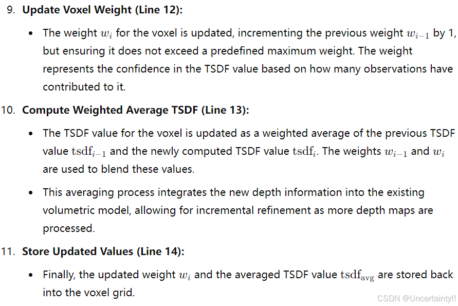通过ICP得到位姿后，我们把每一帧对应的相机坐标系内的体素都转换到了世界坐标系中，每次转换都会对世界坐标系内体素进行更新   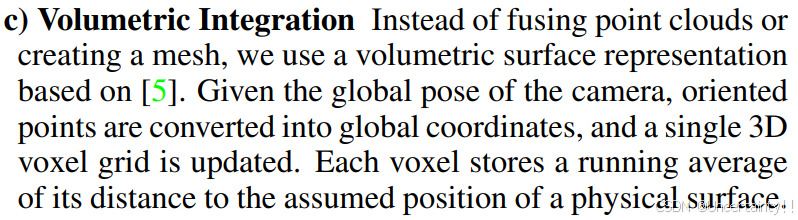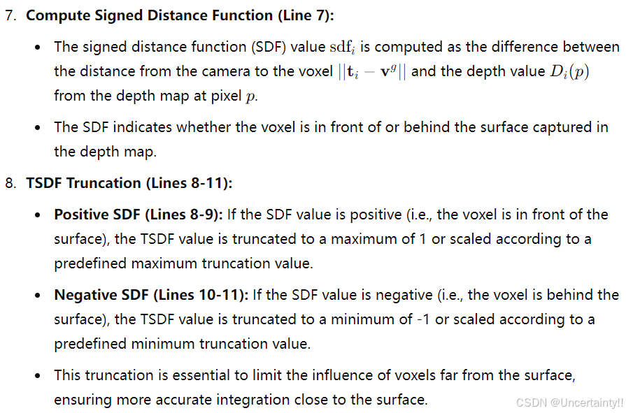论文中提到使用SDF的变体将全局 3D 顶点集成到体素中，指定与实际表面的相对距离。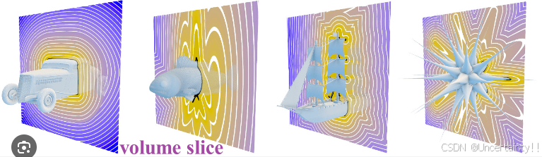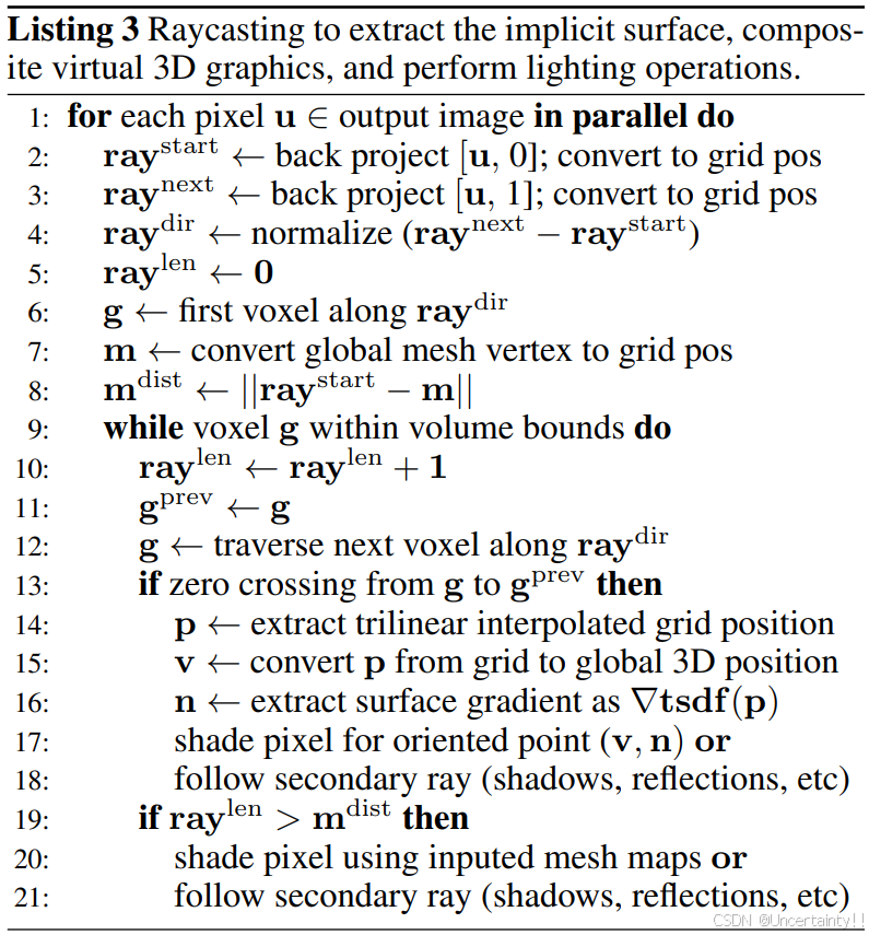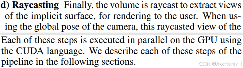这些值在表面前为正，在表面后为负，表面界面由zero-crossing定义，值在此改变符号 下图来自： [截断符号距离 \| TSDF, Truncated Signed Distance Function](http://liuxiao.org/kb/3dvision/3d-reconstruction/tsdf-truncated-signed-distance-function/) SDF计算方式：camera 到 每个 voxel 的距离减去voxel对应的深度  将volume slice (xy plane) 中的每个体素转换到3D位置，而后将这些转换到当前帧（相机坐标系下）用于raycasting后并显示      ### 1.4 Raycasting     ```python Listing 3 Raycasting to extract the implicit surface, composite virtual 3D graphics, and perform lighting operations. 1: for each pixel u ∈ output image in parallel do # For each pixel in the output image, a ray will be cast from the camera's origin through the pixel, # in parallel, meaning each pixel is processed simultaneously. 2: raystart ← back project [u, 0]; convert to grid pos # Compute the starting position of the ray by back-projecting the pixel's coordinates (u, 0) from image space # to the 3D grid (volume) space. This represents the position on the near clipping plane. 3: raynext ← back project [u, 1]; convert to grid pos # Compute a second point on the ray by back-projecting the pixel's coordinates (u, 1) from image space # to 3D grid space. This represents a position further along the viewing direction (typically on the far clipping plane). 4: raydir ← normalize (raynext − raystart) # Calculate the direction of the ray by subtracting the starting point from the next point # and normalizing the resulting vector. 5: raylen ← 0 # Initialize the ray length, which will be used to keep track of how far along the ray we have traveled in the 3D grid. 6: g ← first voxel along raydir # Determine the first voxel in the 3D grid that the ray intersects. This will be the starting voxel for ray traversal. 7: m ← convert global vertex to grid pos # Convert the closest global vertex (from the known surface) to the grid position. This is used to determine # if we need to continue ray traversal or stop and shade the pixel. 8: mdist ← ||raystart − m|| # Calculate the distance from the starting point of the ray to the nearest vertex. # This distance is used to decide if the ray has reached the surface. 9: while voxel g within volume bounds do # While the ray is within the boundaries of the volume (i.e., inside the 3D grid): # This loop traverses the grid along the ray direction. 10: raylen ← raylen + 1 # Increment the ray length as the ray moves from one voxel to the next. 11: gprev ← g # Store the current voxel position before moving to the next one. # This is necessary for detecting zero crossings (surface intersections). 12: g ← traverse next voxel along raydir # Move to the next voxel along the ray's direction. 13: if zero crossing from g to gprev then # Check if there is a zero crossing between the TSDF values of the current voxel and the previous voxel. # A zero crossing indicates that the ray has intersected with the surface. 14: p ← extract trilinear interpolated grid position # Extract the exact intersection point within the grid by performing trilinear interpolation. # This provides a more accurate position of the surface intersection. 15: v ← convert p from grid to global 3D position # Convert the interpolated grid position to a global 3D position. # This gives the exact 3D coordinates of the surface point in the world space. 16: n ← extract surface gradient as ∇tsdf(p) # Compute the surface normal at the intersection point by calculating the gradient of the TSDF (∇tsdf). # The gradient points in the direction of the steepest increase in the TSDF value, representing the surface normal. 17: shade pixel for oriented point (v, n) or # Shade the pixel using the 3D position (v) and the surface normal (n). # This involves computing the pixel's color based on lighting, material properties, and viewing direction. 18: follow secondary ray (shadows, reflections, etc) # Optionally, trace secondary rays to account for shadows, reflections, refractions, etc. # This step can enhance the realism of the rendered image by simulating advanced lighting effects. 19: if raylen > mdist then # If the ray length exceeds the distance to the nearest vertex (mdist), # this implies that the ray has traveled past the expected surface point without finding a zero crossing. 20: shade pixel using inputted maps or # If no zero crossing was detected, use pre-computed maps (e.g., depth maps or normal maps) to shade the pixel. # This fallback ensures that the pixel still gets shaded even if the ray doesn't directly hit the surface. 21: follow secondary ray (shadows, reflections, etc) # Optionally, continue with secondary ray tracing for additional effects like shadows and reflections, as in step 18. ``` ### 1.4 总结一下上述过程