第二十周：机器学习

摘要

ABSTRACT

一、吴恩达机器学习exp2------逻辑回归

1、logistic函数

二、动手深度学习pytorch------数据预处理

摘要

本周接着上周的线性回归，进一步学习了逻辑回归的完整代码，不仅包含了逻辑回归模型的整个训练过程，还对逻辑回归中的损失函数和梯度下降函数进行代码表达。在复习了逻辑回归模型的数学原理后，对其进行代码实践，并且可视化决策边界函数，将自定义模型与库函数自带模型进行准确率、损失函数及其边界函数的比较。最后，接着pytorch动手深度学习的内容，学习了数据预处理部分。

ABSTRACT

This week follows up on last week's linear regression by further studying the complete code for logistic regression, which not only includes the entire training process of a logistic regression model, but also provides a code representation of the loss function and gradient descent function in logistic regression. After reviewing the mathematical principles of the logistic regression model, code practice on it and visualize the decision boundary function, comparing the accuracy, loss function and its boundary function of the custom model with the model that comes with the library function. Finally, the pytorch hands-on deep learning was followed by learning the data preprocessing component.

一、吴恩达机器学习exp2------逻辑回归

1、logistic函数

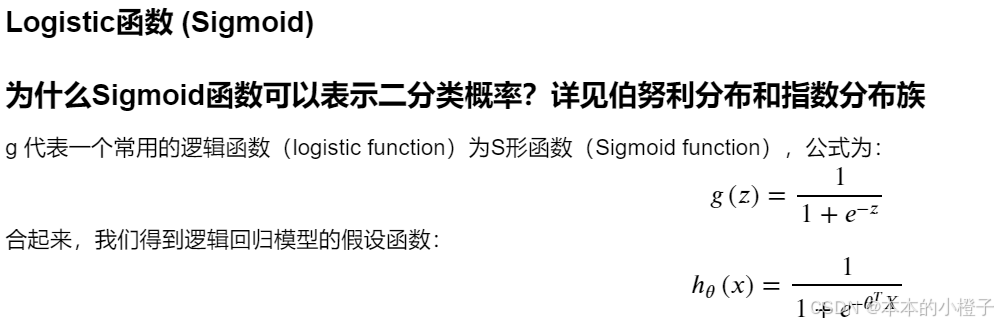
sigmoid函数不仅可以调用scikit-learn 库中自带的LogisticRegression模型，还可以自己定义，自定义及验证如下：

python 复制代码

def sigmoid(z):     #定义sigmoid函数
    return 1 / (1 + np.exp(-z))

#验证sigmoid函数的正确性
nums = np.arange(-10, 10, step=1)  #np.arange()函数返回一个有终点和起点的固定步长的排列
fig, ax = plt.subplots(figsize=(12,8))
ax.plot(nums, sigmoid(nums), 'r')
plt.show()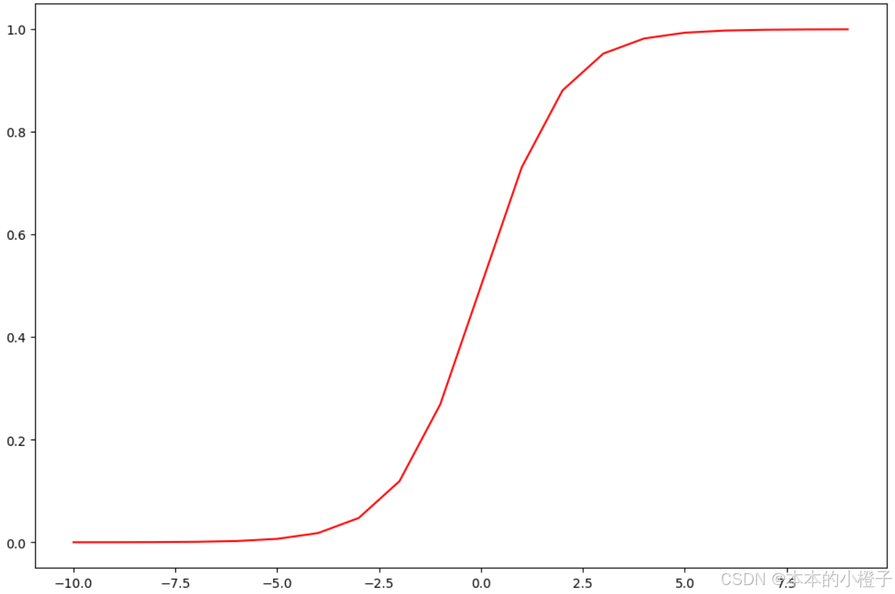

python 复制代码

import time
import matplotlib.pyplot as plt
import numpy as np

from LogisticRegression import sigmoid
nums = np.arange(-5, 5, step=0.1)
fig, ax = plt.subplots(figsize=(12,8))
ax.plot(nums, sigmoid(nums), 'r')
ax.set_title("Sigmoid Function")
ax.grid()
plt.show()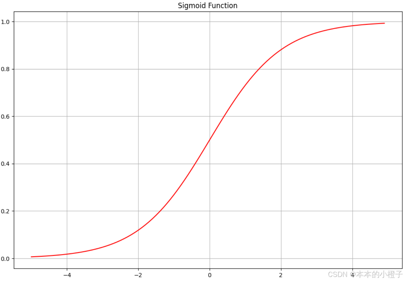

2、数据预处理

加载数据

python 复制代码

import pandas as pd
data = np.loadtxt(fname='ex2data1.txt',delimiter=",")
data = pd.read_csv('ex2data1.txt', header=None, names=['Exam 1', 'Exam 2', 'Admitted'])
data.head()

查看数据集正负样本

python 复制代码

import matplotlib.pyplot as plt
import numpy as np


# 将列表转换为NumPy数组
data = np.array(data)

#绘制数据集正负样本的散点图
fig, ax = plt.subplots(figsize=(12,8))
positive_data_idx= np.where(data[:,2]==1)
positive_data = data[positive_data_idx]
negative_data_idx= np.where(data[:, 2] == 0)
negative_data = data[negative_data_idx]
ax.scatter(x=positive_data[:, 0], y=positive_data[:, 1], s=10, color="red",label="positive")
ax.scatter(x=negative_data[:, 0], y=negative_data[:, 1], s=10, label="negative")
ax.set_title("Dataset")
plt.legend(loc=2)
plt.show()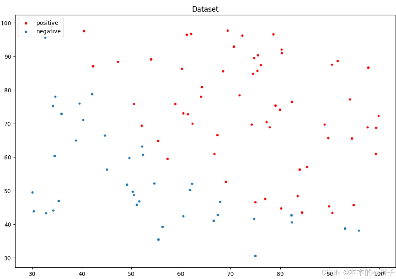

同理，训练集和验证集分别的分布散点图如下：

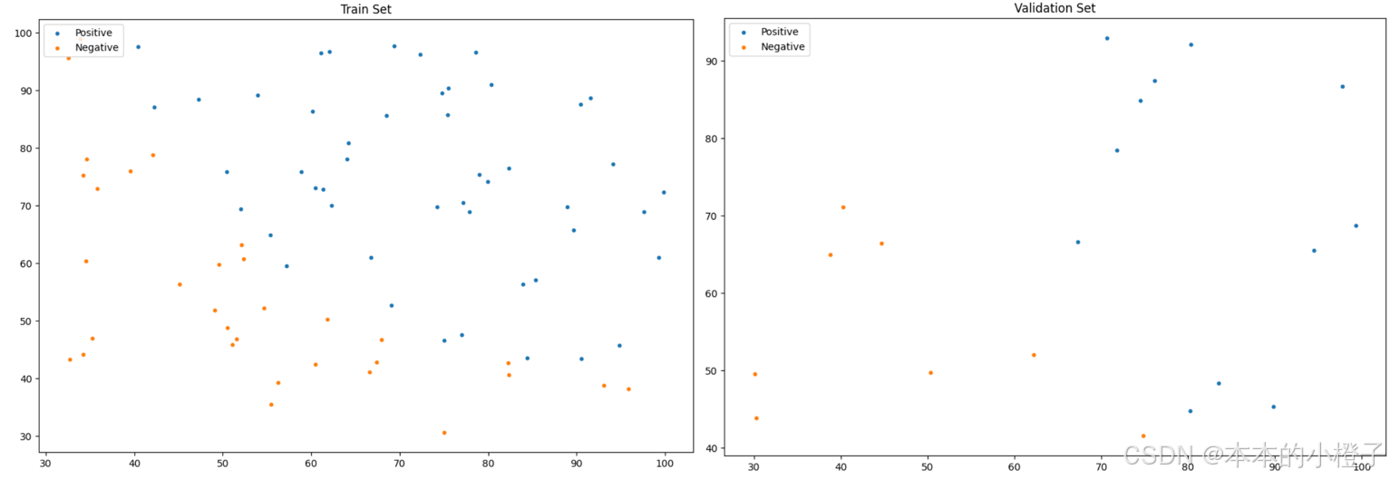
划分训练集额、验证集

python 复制代码

from sklearn.model_selection import train_test_split
train_x, val_x, train_y, val_y = train_test_split(data[:, :-1], data[:, -1], test_size=0.2)
# train_x, val_x, train_y, val_y = data[:, :-1], data[:, :-1], data[:, -1], data[:, -1]

#绘制数据集中训练集和验证集的各个分数段的分布散点图
fig, ax = plt.subplots(figsize=(12,8))
ax.scatter(x=train_x[:,0], y=train_x[:,1], s=10, label="Train")
ax.scatter(x=val_x[:,0], y=val_x[:,1], s=10, color="red", label="Validation")
ax.set_title('Dataset for Train and Validation')
ax.legend(loc=2)
plt.show()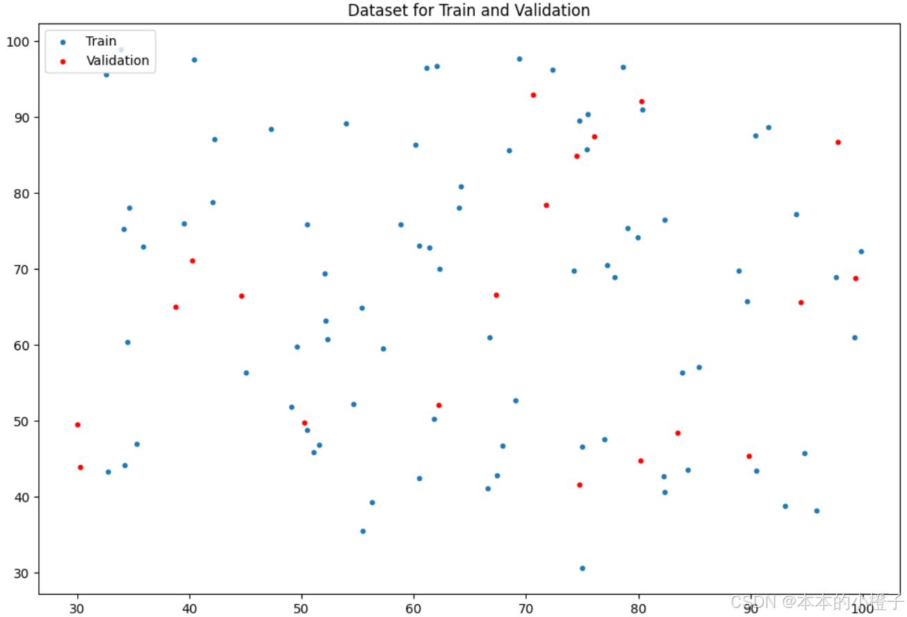

3、损失函数

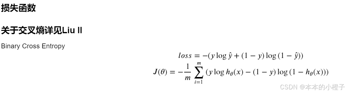
定义损失函数

python 复制代码

def cost(theta, X, y):
    theta = np.matrix(theta)
    X = np.matrix(X)
    y = np.matrix(y)
    first = np.multiply(-y, np.log(sigmoid(X * theta.T)))#这个是(100,1)乘以(100,1)就是对应相乘
    second = np.multiply((1 - y), np.log(1 - sigmoid(X * theta.T)))
    return np.sum(first - second) / (len(X))

初始化参数

python 复制代码

data.insert(0, 'Ones', 1)  #增加一列，使得矩阵相乘更容易

cols = data.shape[1]
X = data.iloc[:,0:cols-1] #训练数据
y = data.iloc[:,cols-1:cols]#标签

#将X、y转化为数组格式
X = np.array(X.values)
y = np.array(y.values)
theta = np.zeros(3)  #初始化向量theta为0
theta,X,y

检查矩阵属性和当前损失

python 复制代码

X.shape, theta.shape, y.shape
cost(theta, X, y)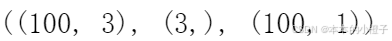

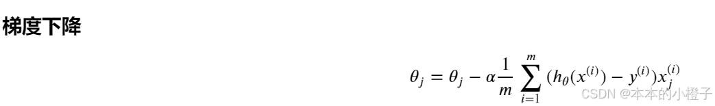
4、梯度下降

定义梯度下降函数

python 复制代码

def gradient(theta, X, y):  #梯度下降
    theta = np.matrix(theta)    #将参数theta、特征值X和标签y转化为矩阵形式
    X = np.matrix(X)
    y = np.matrix(y)
    
    parameters = int(theta.ravel().shape[1])    #.ravel()将数组维度拉成一维数组,  .shape()是长度，parameters指theta的下标个数
    grad = np.zeros(parameters) 
    
    error = sigmoid(X * theta.T) - y  #误差
    
    for i in range(parameters):    #迭代的计算梯度下降
        term = np.multiply(error, X[:,i])
        grad[i] = np.sum(term) / len(X)
  
    return grad

gradient(theta, X, y)

最优化

python 复制代码

import scipy.optimize as opt
result = opt.fmin_tnc(func=cost, x0=theta, fprime=gradient, args=(X, y))#opt.fmin_tnc（）函数用于最优化
result

最优化后的损失

python 复制代码

cost(result[0], X, y)

以上的1、2、3、4条都是可以自定义的函数模块，把很多个功能封装到LogisticRegression类中，后面逻辑回归的训练过程就是直接调用其内部的函数即可。

5、设定评价指标

定义准确率函数

python 复制代码

def predict(theta, X):   #准确率
    probability = sigmoid(X * theta.T)
    return [1 if x >= 0.5 else 0 for x in probability]

theta_min = np.matrix(result[0])
predictions = predict(theta_min, X)
correct = [1 if ((a == 1 and b == 1) or (a == 0 and b == 0)) else 0 for (a, b) in zip(predictions, y)]#zip 可以同时比较两个列表
accuracy = (sum(map(int, correct)) % len(correct))#map会对列表correct的每个元素调用int函数，将其转换成一个整数，然后返回一个迭代器，可以用来迭代所有转换后的结果
print ('accuracy = {0}%'.format(accuracy))  #因为数据总共100 个所以准确率只加测对的就行不用除了

查看精确度、损失和F1-score

php 复制代码

acc = logistic_reg.test(val_x,val_y_ex)
print("Accuracy on Test Set: {:.2f}%".format(acc * 100))
from sklearn.metrics import f1_score
f1 = f1_score(y_true=val_y_ex,y_pred=logistic_reg.predict(val_x))
print("My F1 Score: {:.4f}".format(f1))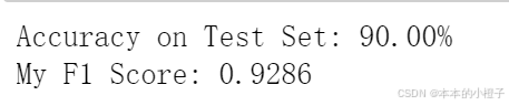

调用库函数进行验证

python 复制代码

from sklearn.linear_model import LogisticRegression
sk_lr = LogisticRegression(max_iter=50000)
sk_lr.fit(train_x,train_y)
sk_pred = sk_lr.predict(val_x)
count = np.sum(np.equal(sk_pred,val_y))
sk_acc = count/val_y.shape[0]
sk_prob = sk_lr.predict_proba(val_x)

from LogisticRegression import bce_loss
sk_loss = bce_loss(sk_prob[:,1], val_y_ex)
sk_theta = np.array([[sk_lr.intercept_[0],sk_lr.coef_[0,0],sk_lr.coef_[0,1]]])
sk_f1 = f1_score(y_true=val_y_ex,y_pred=sk_pred)
print("Sklearn Accuracy: {:.2f}%".format(sk_acc * 100))
print("Sklearn Val Loss: {:.4f}".format(sk_loss))
print("SKlearn Parameters: ",sk_theta)
print("Sklearn F1 Score: {:.4f}".format(sk_f1))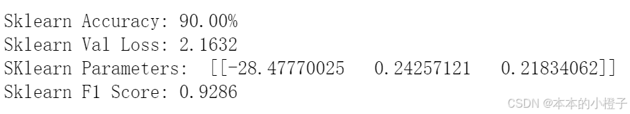

6、决策边界

绘制决策边界函数

python 复制代码

#计算系数:结果是2*3维数组
coef = -(theta/ theta[0, 2])
coef1 = -(sk_theta / sk_theta[0, 2])


data = data.to_numpy()  # 将dataframe形式的数据转化为numpy形式: 使用.to_numpy()方法

x = np.arange(0,100, step=10)   #x轴是等距刻度
y = coef[0,0] + coef[0,1]*x   #y是自定义边界函数
y1 = coef1[0,0] + coef[0,1]*x  #y1是调用边界函数

#绘制边界函数
fig, ax = plt.subplots(figsize=(12,8))
ax.plot(x,y,label="My Prediction",color='purple')
ax.plot(x,y1,label="Sklearn",color='orange')

#绘制散点图
ax.scatter(x=positive_data[:, 0], y=positive_data[:, 1], s=10, color="red",label="positive")
ax.scatter(x=negative_data[:, 0], y=negative_data[:, 1], s=10, color="blue",label="negative")
ax.set_title("Decision Boundary")
plt.legend(loc=2)
plt.show()

绘制训练过程

记录每一轮的损失值

python 复制代码

fig, ax = plt.subplots(figsize=(12,8))
ax.plot(np.arange(1,epochs+1), train_loss, 'r', label="Train Loss")
ax.plot(np.arange(1,epochs+1), val_loss, 'b', label="Val Loss")
ax.set_xlabel('Epoch')
ax.set_ylabel('Loss')
ax.set_title('Train Curve')
plt.legend(loc=2)
plt.show()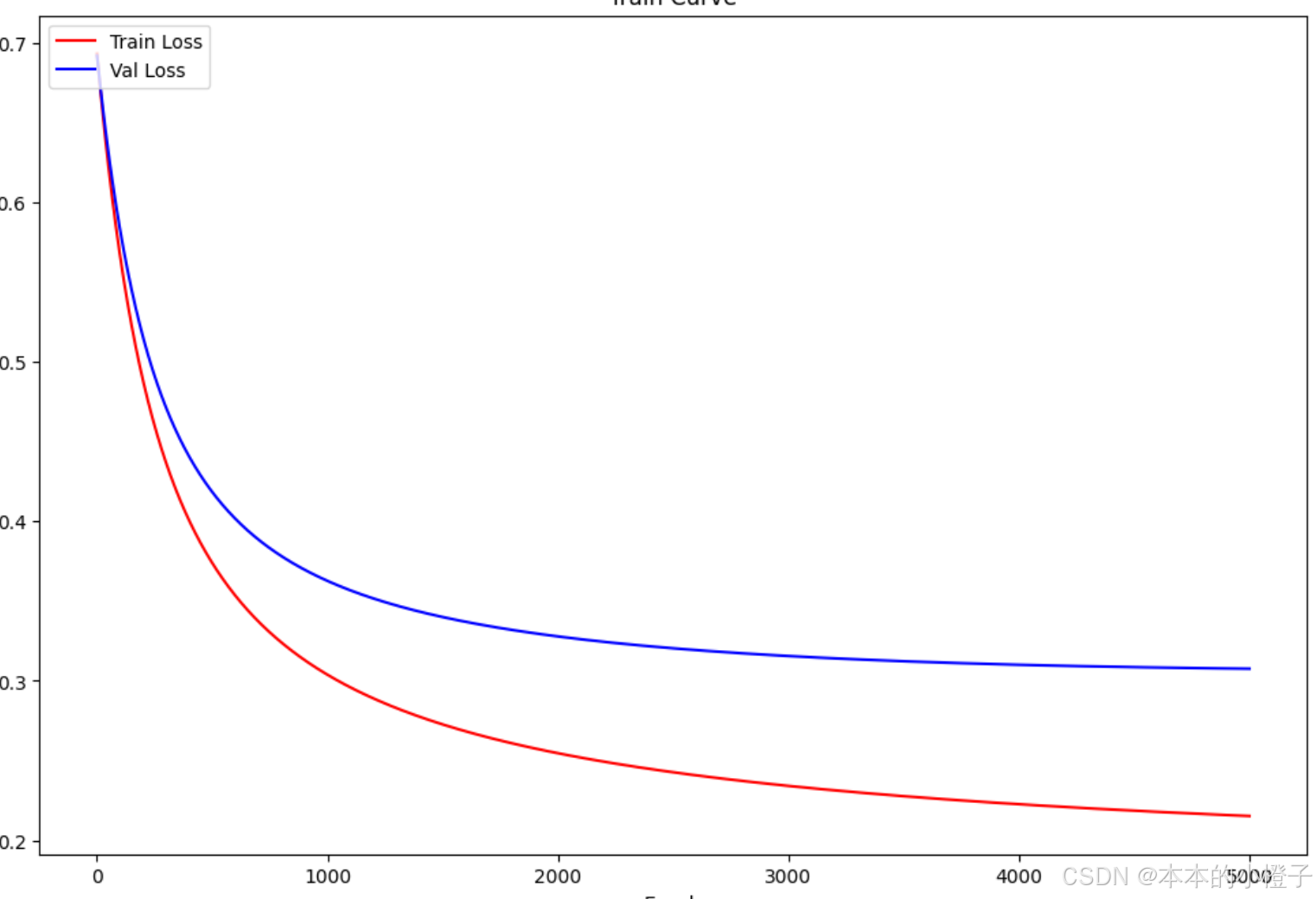

7、正则化

正则化实际上就是对损失函数及梯度下降的一种改进方式，它在其他数据预处理、训练过程及结果可视化的方面都都跟普通的逻辑回归没什么差别。下面仅指出不同的地方进行修改

正则化损失函数

相比于正常的损失函数，多了一个正则项reg

python 复制代码

#正则化代价函数
def costReg(theta, X, y, learningRate):

    theta = np.matrix(theta)
    X = np.matrix(X)
    y = np.matrix(y)

    first = np.multiply(-y, np.log(sigmoid(X * theta.T)))
    second = np.multiply((1 - y), np.log(1 - sigmoid(X * theta.T)))
    reg = (learningRate / (2 * len(X))) * np.sum(np.power(theta[:,1:theta.shape[1]], 2))#注意下标 j是从1开始到n的  不包含0
    return np.sum(first - second) / len(X) + reg

正则化梯度下降

在迭代的计算梯度的时候，如果是第一次计算梯度就不需要加正则化项，其余轮次需要加上正则化项

python 复制代码

#正则化梯度下降
def gradientReg(theta, X, y, learningRate):
    theta = np.matrix(theta)
    X = np.matrix(X)
    y = np.matrix(y)
    
    parameters = int(theta.ravel().shape[1])
    grad = np.zeros(parameters)
    
    error = sigmoid(X * theta.T) - y
    
    for i in range(parameters):
        term = np.multiply(error, X[:,i])
        
        if (i == 0):
            grad[i] = np.sum(term) / len(X) #和上文一样，我们这里没有执行梯度下降，我们仅仅在计算一个梯度步长
        else:
            grad[i] = (np.sum(term) / len(X)) + ((learningRate / len(X)) * theta[:,i])
    
    return grad

决策边界可视化

python 复制代码

fig, ax = plt.subplots(figsize=(12,8))

# 使用更鲜明的颜色和更小的点
ax.plot(x, y, label="My Prediction", color='purple', linestyle='--')  # 虚线
ax.plot(x, y1, label="Sklearn", color='orange', linestyle=':')  # 点线
# ax.scatter(x=my_bd[:, 0], y=my_bd[:, 1], s=5, color="yellow", edgecolor='black', label="My Decision Boundary")
# ax.scatter(x=sk_bd[:, 0], y=sk_bd[:, 1], s=5, color="gray", edgecolor='black', label="Sklearn Decision Boundary")

# 保持正负样本点的颜色鲜艳，但可以适当减小大小
ax.scatter(x=positive_data[:, 0], y=positive_data[:, 1], s=20, color="red", label="positive")
ax.scatter(x=negative_data[:, 0], y=negative_data[:, 1], s=20, color="blue", label="negative")

ax.set_title('Decision Boundary')
ax.legend(loc=2)
plt.show()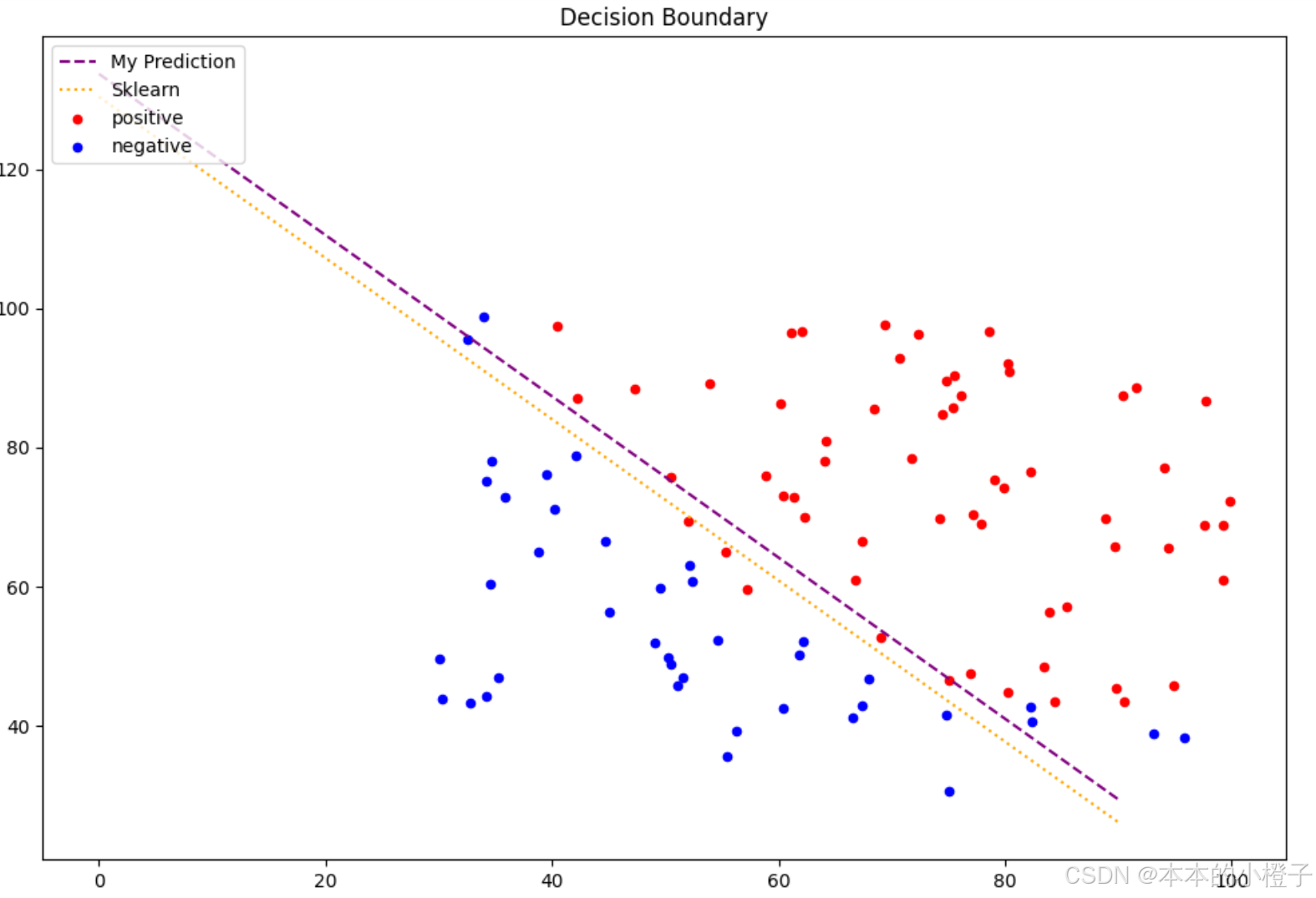

二、动手深度学习pytorch------数据预处理

1、数据集读取

创建一个人工数据集，并存储在CSV（逗号分隔值）文件

python 复制代码

os.makedirs(os.path.join('..', 'data'), exist_ok=True)
data_file = os.path.join('..', 'data', 'house_tiny.csv')
with open(data_file, 'w') as f:
    f.write('NumRooms,Alley,Price\n')
    f.write('NA,Pave,127500\n')
    f.write('2,NA,106000\n')
    f.write('4,NA,178100\n')
    f.write('NA,NA,140000\n')

从创建的CSV文件中加载原始数据集

python 复制代码

import pandas as pd

data = pd.read_csv(data_file)
print(data)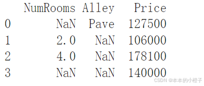

2、缺失值处理

处理缺失值的方法有插值法和删除法，下面代码以插值法为例

python 复制代码

inputs, outputs = data.iloc[:, 0:2], data.iloc[:, 2]
inputs = inputs.fillna(inputs.mean())
print(inputs)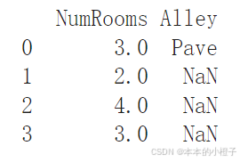

3、转换为张量格式

python 复制代码

import torch

X = torch.tensor(inputs.to_numpy(dtype=float))
y = torch.tensor(outputs.to_numpy(dtype=float))
X, y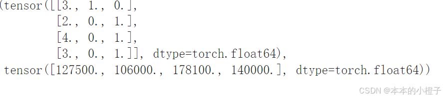

总结

本周继续完成吴恩达机器学习的实验2部分------逻辑回归，并且复习了对应的理论知识，对交叉熵、梯度更新、正则化表示的数学原理进行推导并且实现在代码上；pytorch学习了数据集的读取、缺失值的处理以及张量格式的转换。下周继续完成吴恩达实验，并接着学习pytorch比较细致的知识点。