图解Transfomer（上）

We will look at The Transformer -- a model that uses attention to boost the speed with which these models can be trained.

Transformer使用Attention机制加速模型训练。

传统的RNN或者LSTM都是串行处理句子中的每个单词，而Attention可以并行计算句子中各个单词的关系。
Attention的并行计算可以充分利用GPU/TPU的并行计算能力。

The Transformer was proposed in the paper Attention is All You Need. A TensorFlow implementation of it is available as a part of the Tensor2Tensor package. Harvard's NLP group created a guide annotating the paper with PyTorch implementation.

在论文《Attention is All You Need》中首次提出了Transformer。针对Transformer有两种实现：基于TensorFlow和PyTorch的实现。其中Harvard在2022年又重写了一篇文章解释Transformer以及代码实现：The Annotated Transformer

A High-Level Look

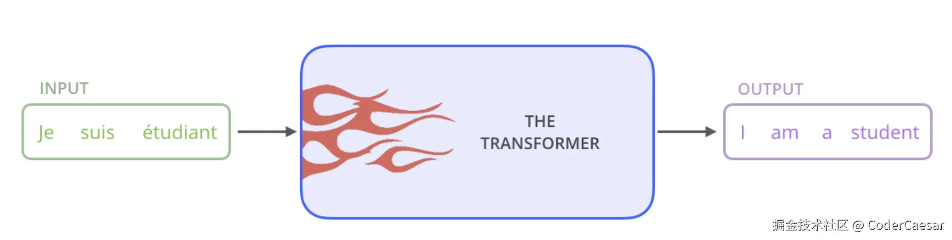
先将TRANSFORMER当成一个黑盒，让其完成将法语翻译成英语的任务。

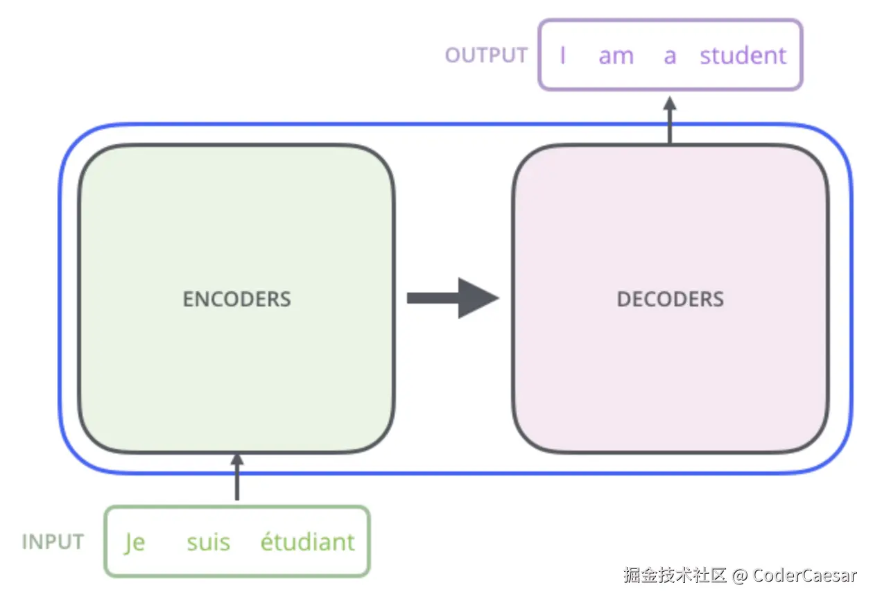
先简单看下黑盒TRANSFORMER的结构：由6层ENCODER组成的ENCODERS和由6层DECODER组成的DECODERS。

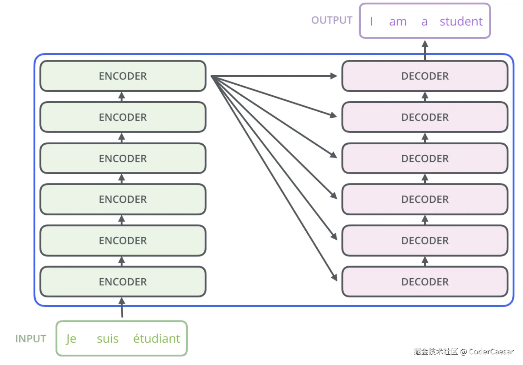
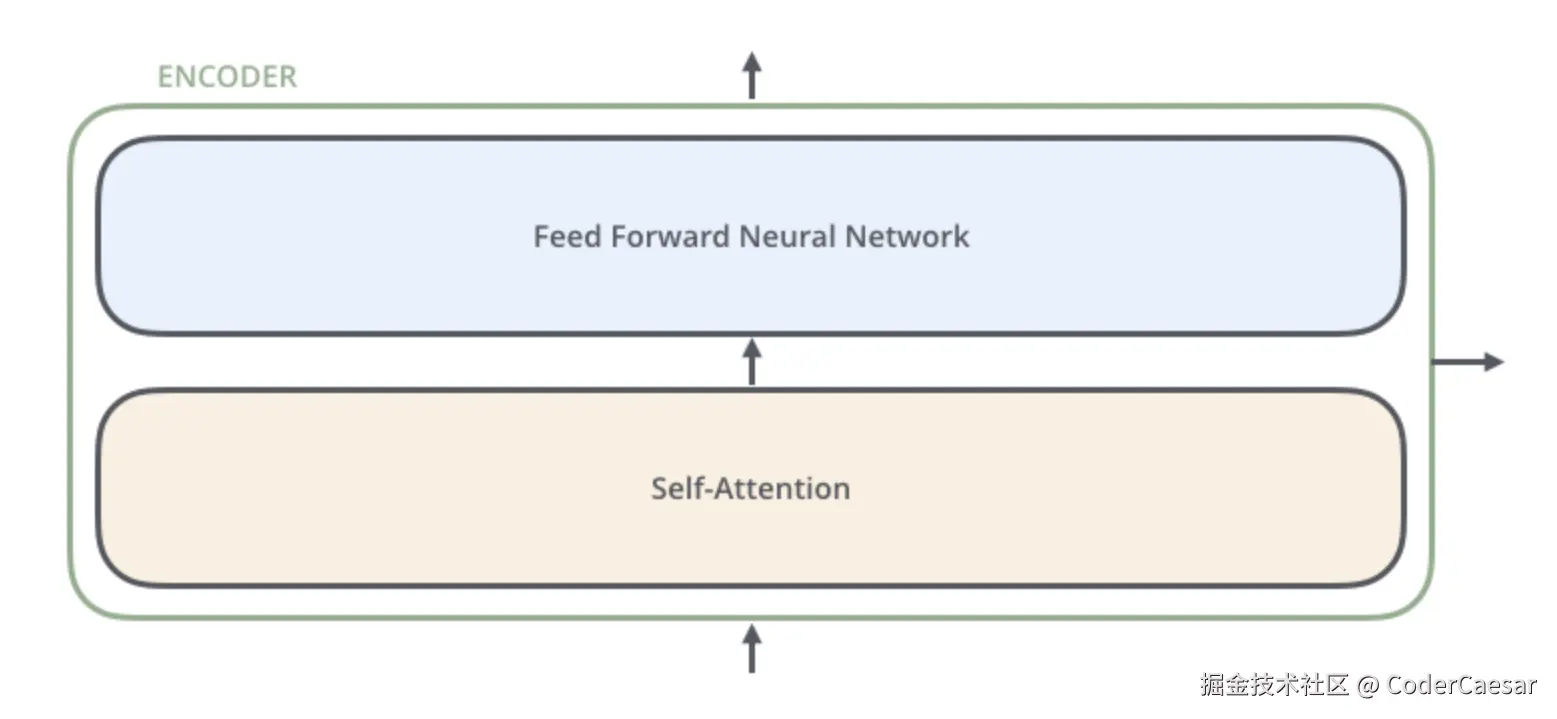
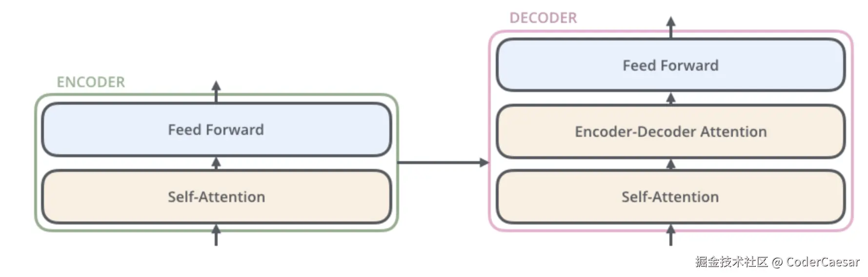
再拆解下ENCODER层，每个ENCODER的结构都是一样的，且ENCODER之间不共享权重参数。每个ENCODER由两层组成：

Self-Attention层：ENCODER的输入首先流入Self-Attention层，在编码一个单词时，会同时考虑句子中的其他单词。
Feed Forward Neural Network：Self-Attention的结果流入Feed Forward Neural Network。完全相同的前馈神经网络会被独立的应用于每一个位置。

DECODER层也有Self-Attention层和Feed Forward层，只是在这两层之间增加了Encoder-Decoder Attention层。

Tensor流转

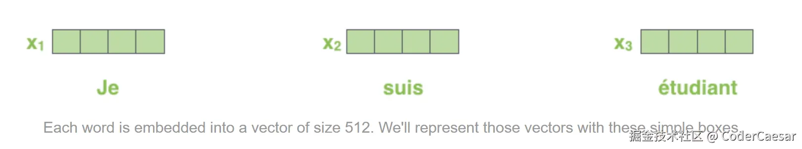
首先将待翻译句子的每个单词转成512维的词向量。

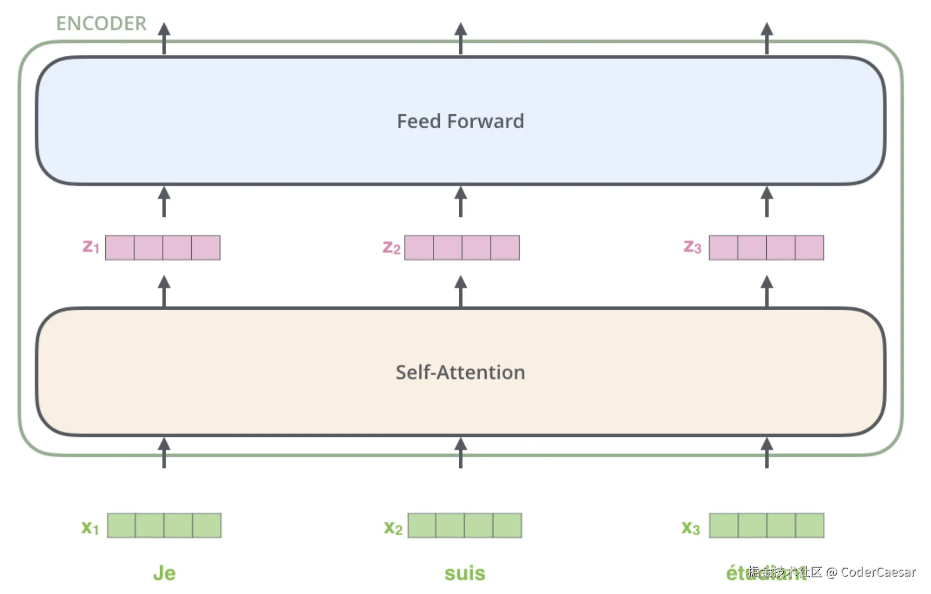
这些词向量将流经ENCODER的两层：Self-Attention和Feed Forward。

Here we begin to see one key property of the Transformer, which is that the word in each position flows through its own path in the encoder. There are dependencies between these paths in the self-attention layer. The feed-forward layer does not have those dependencies, however, and thus the various paths can be executed in parallel while flowing through the feed-forward layer.

Transformer的关键特性：在encoder中每个位置的word流经各自的路径。在self-attention层，这些路径间有依赖，但是当流经Feed Forward时，路径间就不再有依赖了，也就是说，这些路径可以在feed-forward层并行处理。这提高了模型的训练效率。

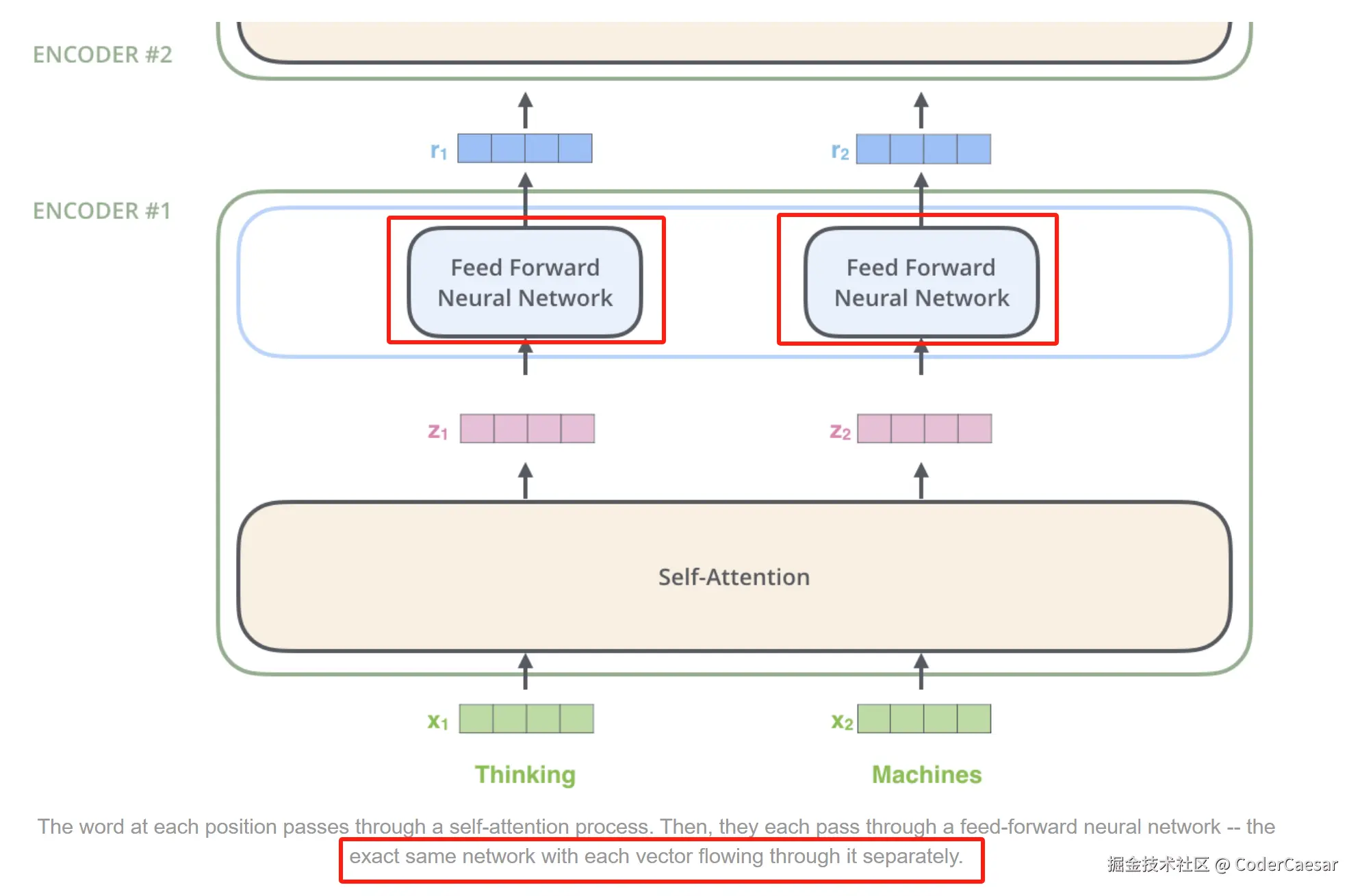
每个单词在feed-forward层有完全一样而又独立的Feed Forward Neural Network。词向量流经ENCODER#1之后的输出，流入到了ENCODER#2。

Self-Attention at a High Level

"The animal didn't cross the street because it was too tired"

上面这句话中的 it 指代的是 the animal，还是 the street。对于人类来说很简单，但是对于计算机算法来说不那么简答。

当模型处理单词 it 时，attention机制可以将 it 与 animal 关联起来。

As the model processes each word (each position in the input sequence), self attention allows it to look at other positions in the input sequence for clues that can help lead to a better encoding for this word.

当模型处理每个单词（句子中的每个位置）时，self attention可以从句子中其他位置找到线索，以更好的编码这个单词。

If you're familiar with RNNs, think of how maintaining a hidden state allows an RNN to incorporate its representation of previous words/vectors it has processed with the current one it's processing. Self-attention is the method the Transformer uses to bake the "understanding" of other relevant words into the one we're currently processing.

上面这段话，非常清楚的说明了RNN与 self-attention 在处理长距离依赖中的不同：RNN通过串行的方式逐层传递之前处理过的words/vectors，在传递过程中有信息的丢失（考虑下LSTM中的forget gate）；但是self-attention完全摒弃了这种依赖传递，总是能将与当前词相关的单词理解应用到当前词的处理中。

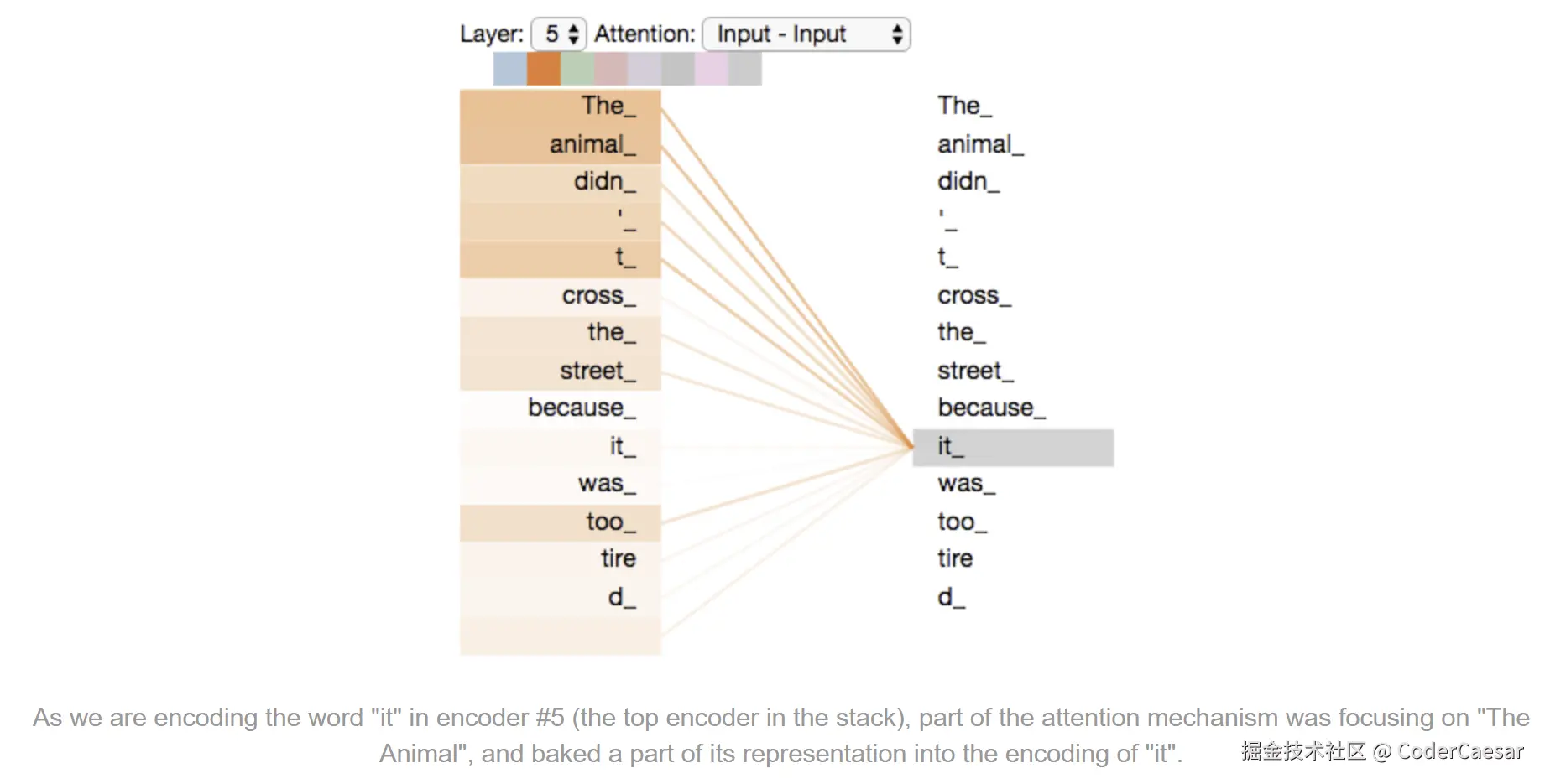
通过上图的"热力图"，可以看到 it 与 "the animal" 的关系权重最大。

Self-Attention in Detail

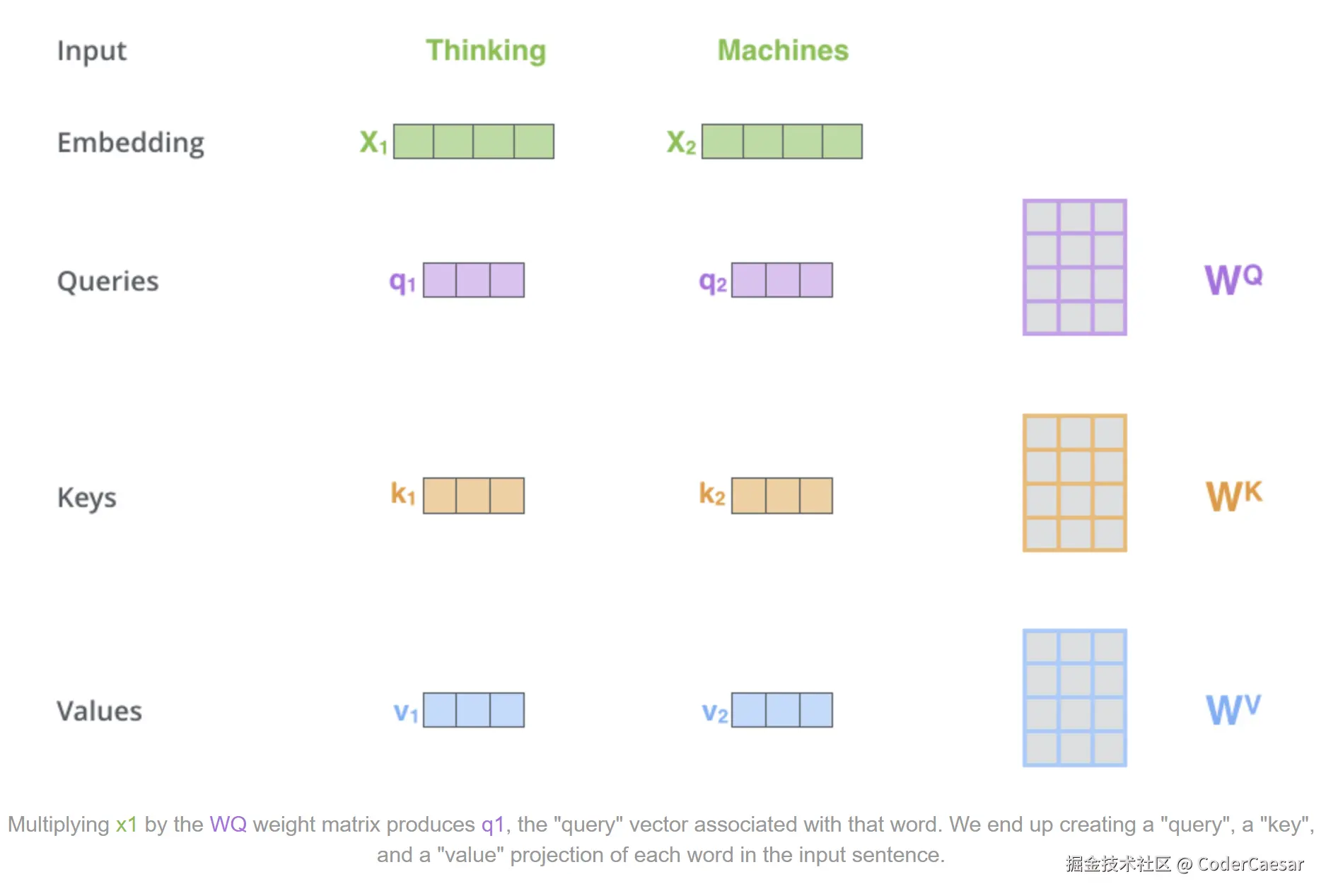
在训练过程中，给定参数矩阵 <math xmlns="http://www.w3.org/1998/Math/MathML"> W Q , W K , W V W^Q, W^K, W^V </math>WQ,WK,WV 。

第一步 ：每个 Embedding 向量分别左乘 <math xmlns="http://www.w3.org/1998/Math/MathML"> W Q , W K , W V W^Q, W^K, W^V </math>WQ,WK,WV，计算得到 Query vector，Key vector，Value vector。

Notice that these new vectors are smaller in dimension than the embedding vector. Their dimensionality is 64, while the embedding and encoder input/output vectors have dimensionality of 512. They don't HAVE to be smaller, this is an architecture choice to make the computation of multiheaded attention (mostly) constant.

需要注意的是，Query Ke Value vector的维度（通常是64维）比 embedding vector的维度要小（通常是512维）。其实维度不是必须要比 embedding vector的维度小，只是这么做（一种架构性选择）可以在多头注意力机制中使得计算常量话，计算（在很大程度上）保持恒定。

The second step in calculating self-attention is to calculate a score. Say we're calculating the self-attention for the first word in this example, "Thinking". We need to score each word of the input sentence against this word. The score determines how much focus to place on other parts of the input sentence as we encode a word at a certain position.

第二步 ：计算一个分值。假设我们要 ENCODE 第一个单词 Thinking，需要计算其他单词与这个单词的分值。这个分值表示当我们 ENCODE 这个单词 Thinking 时，我们需要多大程度的关注句子中的其他单词。

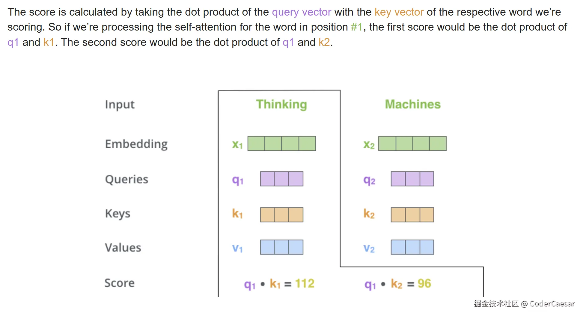
通过 Query vector 点乘 Key vector来得到分值。

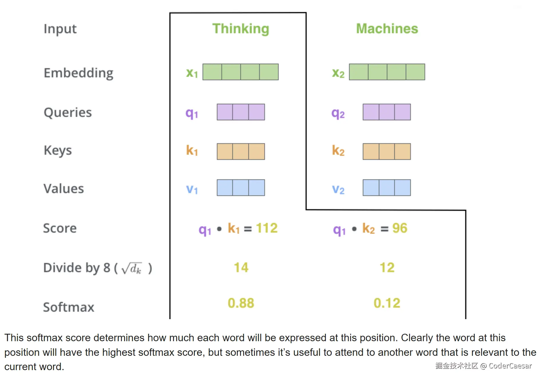
第三、第四步，对第二步中求得分值除以8（the square root of the dimension of the key vectors used in the paper -- 64. This leads to having more stable gradients更稳定的梯度. There could be other possible values here, but this is the default。key向量维数的平方根），然后通过 softmax 进行归一化。

softmax

标准公式

给定一个输入向量 <math xmlns="http://www.w3.org/1998/Math/MathML"> z = [ z 1 , z 2 , . . . , z n ] \mathbf{z} = [z_1, z_2, ..., z_n] </math>z=[z1,z2,...,zn]，Softmax 对每个元素 <math xmlns="http://www.w3.org/1998/Math/MathML"> z i z_i </math>zi 的计算为：
<math xmlns="http://www.w3.org/1998/Math/MathML" display="block"> Softmax ( z i ) = e z i ∑ j = 1 n e z j \text{Softmax}(z_i) = \frac{e^{z_i}}{\sum_{j=1}^n e^{z_j}} </math>Softmax(zi)=∑j=1nezjezi

其中：

<math xmlns="http://www.w3.org/1998/Math/MathML"> e z i e^{z_i} </math>ezi：对 <math xmlns="http://www.w3.org/1998/Math/MathML"> z i z_i </math>zi 取指数（确保结果为正）。
分母 <math xmlns="http://www.w3.org/1998/Math/MathML"> ∑ j = 1 n e z j \sum_{j=1}^n e^{z_j} </math>∑j=1nezj：所有元素的指数和（保证概率归一化，总和为 1）。

特性

输出范围 ：每个 <math xmlns="http://www.w3.org/1998/Math/MathML"> Softmax ( z i ) ∈ ( 0 , 1 ) \text{Softmax}(z_i) \in (0, 1) </math>Softmax(zi)∈(0,1)，且总和为 1。
放大最大值：Softmax 会强化最大值的概率。

python实现

python 复制代码

import numpy as np

x = np.array([14, 12])
softmax = np.exp(x) / np.sum(np.exp(x))
print(softmax)  # 输出: [0.88079708 0.11920292]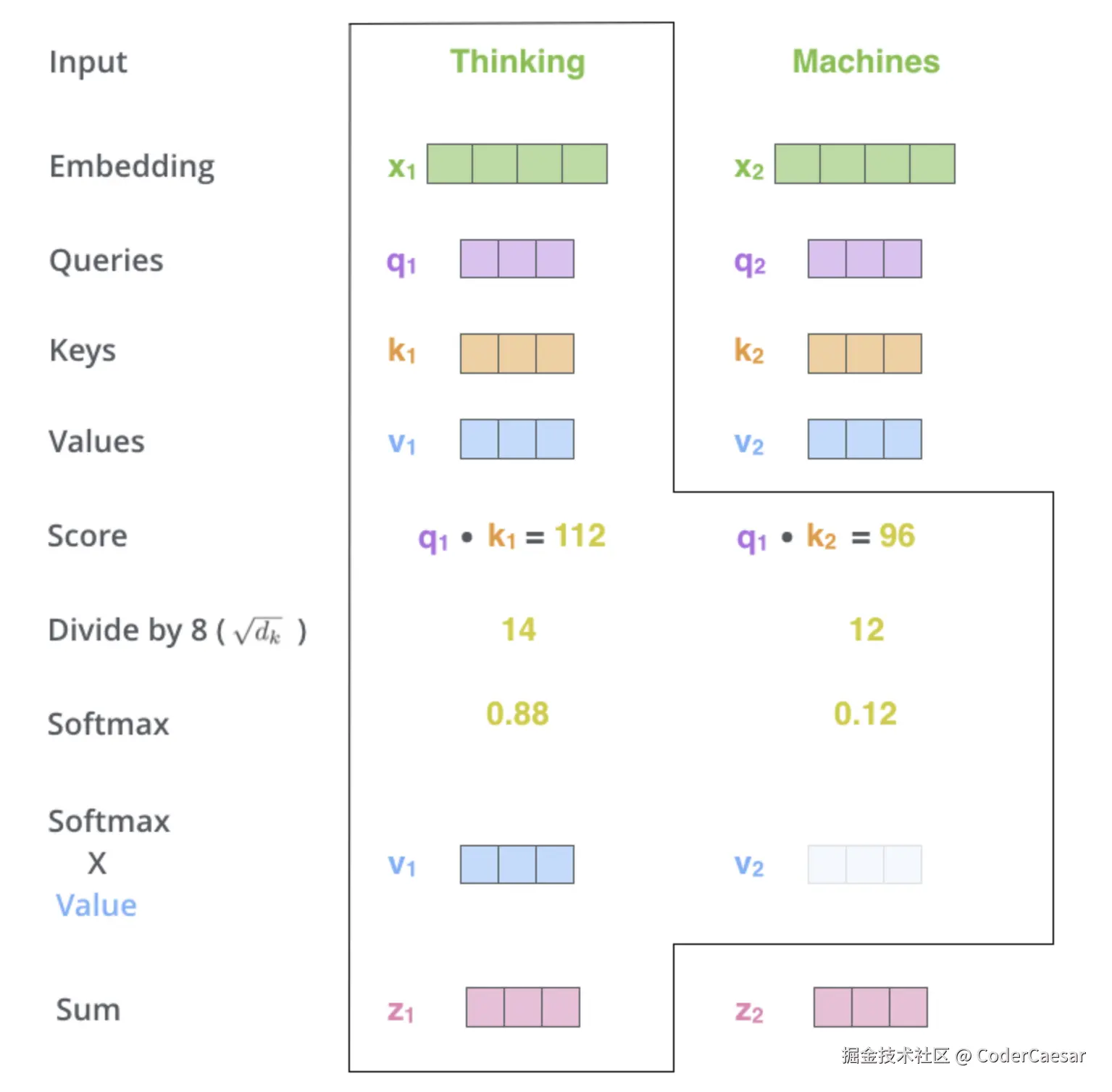

第五步：用上一步得到的 Softmax 乘以 Value vector，为下一步的累加做准备。

The fifth step is to multiply each value vector by the softmax score (in preparation to sum them up). The intuition here is to keep intact the values of the word(s) we want to focus on, and drown-out irrelevant words (by multiplying them by tiny numbers like 0.001, for example).

第五步直观上理解：突出关键信息，抑制无关信息。

第六步 ：The sixth step is to sum up the weighted value vectors. This produces the output of the self-attention layer at this position (for the first word). <math xmlns="http://www.w3.org/1998/Math/MathML"> z 1 = 0.88 v 1 + 0.12 v 2 \mathbf{z}_1 = 0.88 \mathbf{v}_1 + 0.12 \mathbf{v}_2 </math>z1=0.88v1+0.12v2 这样就得到了当前单词的 seft-attention 输出。

Matrix Calculation of Self-Attention

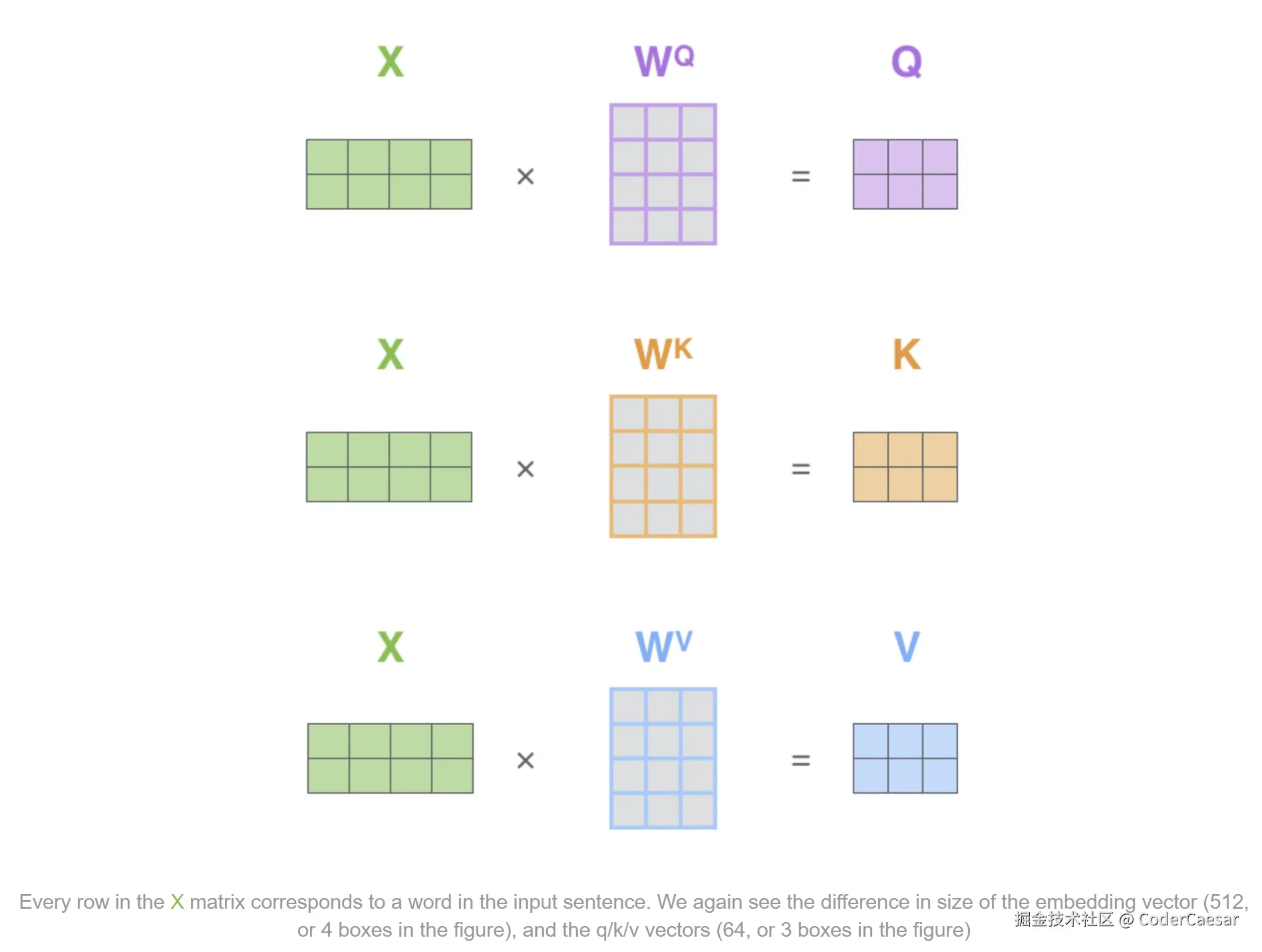
第一步 ：计算Query Key Value矩阵。X矩阵的每一行表示句子中的每个单词。 <math xmlns="http://www.w3.org/1998/Math/MathML"> W Q , W K , W V W^Q, W^K, W^V </math>WQ,WK,WV 是训练过程中的参数矩阵。

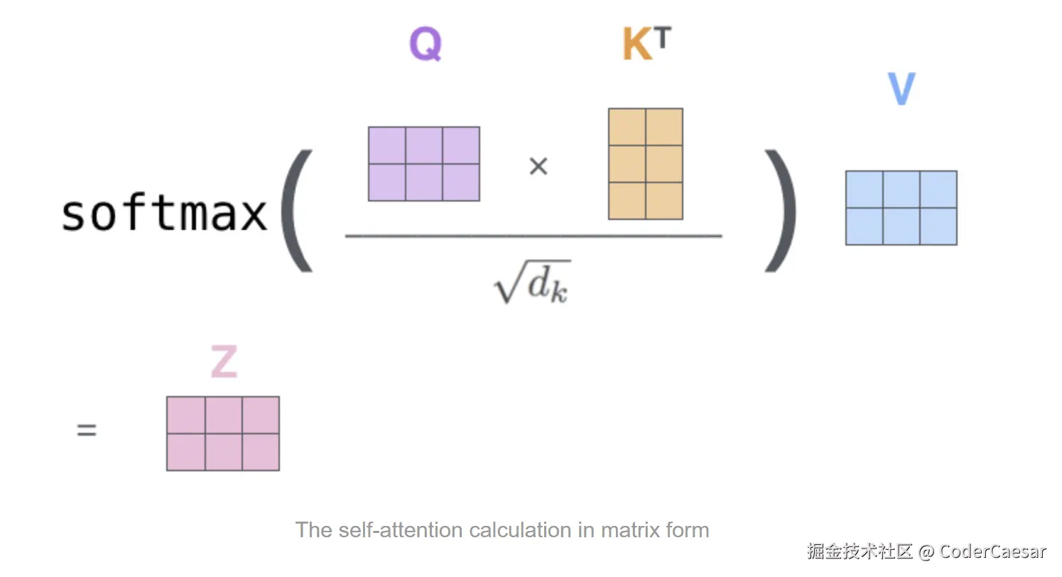
最后一步 ：通过一个公式获得结果。注意 <math xmlns="http://www.w3.org/1998/Math/MathML"> K T \mathbf{K}^T </math>KT 表示的是矩阵转置。

The Beast With Many Heads

beast 怪兽、野兽、猛兽

The paper further refined the self-attention layer by adding a mechanism called "multi-headed" attention. This improves the performance of the attention layer in two ways:

It expands the model's ability to focus on different positions. Yes, in the example above, z1 contains a little bit of every other encoding, but it could be dominated by the actual word itself. If we're translating a sentence like "The animal didn't cross the street because it was too tired", it would be useful to know which word "it" refers to.

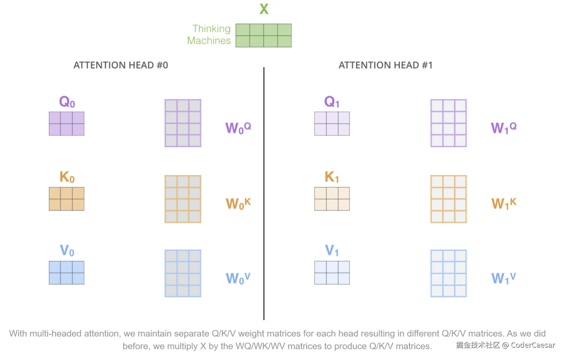
It gives the attention layer multiple "representation subspaces". As we'll see next, with multi-headed attention we have not only one, but multiple sets of Query/Key/Value weight matrices (the Transformer uses eight attention heads, so we end up with eight sets for each encoder/decoder). Each of these sets is randomly initialized. Then, after training, each set is used to project the input embeddings (or vectors from lower encoders/decoders) into a different representation subspace.

通过 "multi-headed" attention 多头注意力机制增强 self-attention层的性能：

增强了模型聚焦于不同位置的能力。比如当我们翻译 "The animal didn't cross the street because it was too tired"时，当遇到 it 时，通过多头注意力机制，可以很容易知道 it 指代的是 "The animal"。
为注意力层提供了多个表示子空间。默认提供8组随机的权重参数矩阵 <math xmlns="http://www.w3.org/1998/Math/MathML"> W Q , W K , W V W^Q, W^K, W^V </math>WQ,WK,WV ，获得8组不同的词向量。

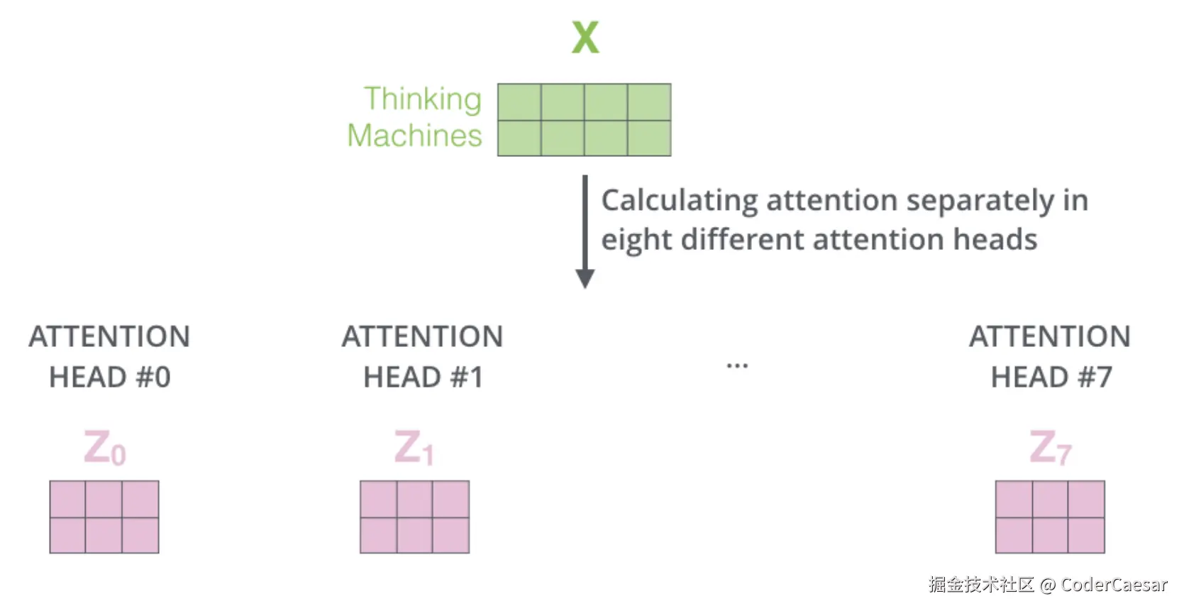
在8个不同的attention head中，分别计算attention。

通过上面的计算，attention层得到了8个attention矩阵数据，但是Feed Forward Neural Network需要的是一个矩阵（每一行代表一个单词），因此需要对这8个矩阵数据做一下变化：

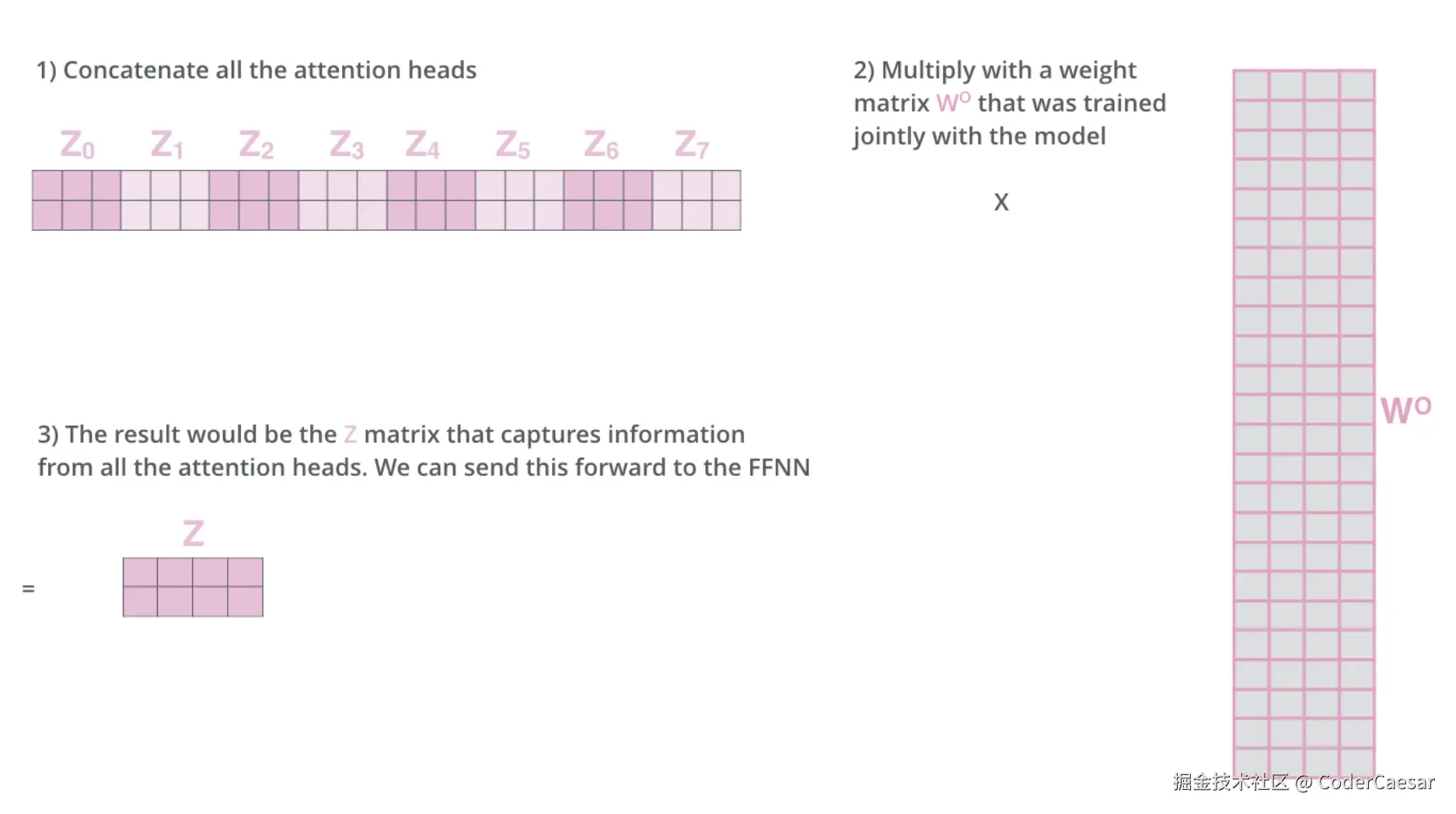
将 <math xmlns="http://www.w3.org/1998/Math/MathML"> Z 0 , Z 1 , ⋯ , Z 7 \mathbf{Z}_0, \mathbf{Z}_1, \cdots, \mathbf{Z}_7 </math>Z0,Z1,⋯,Z7 拼接成一个矩阵
用拼接的矩阵乘以通过训练得到的权重矩阵 <math xmlns="http://www.w3.org/1998/Math/MathML"> W o \mathbf{W}^o </math>Wo
得到的结果 <math xmlns="http://www.w3.org/1998/Math/MathML"> Z \mathbf{Z} </math>Z 就是包含了所有 attention head的信息矩阵，可以直接流转到 Feed Forward Neural Network（FFNN）

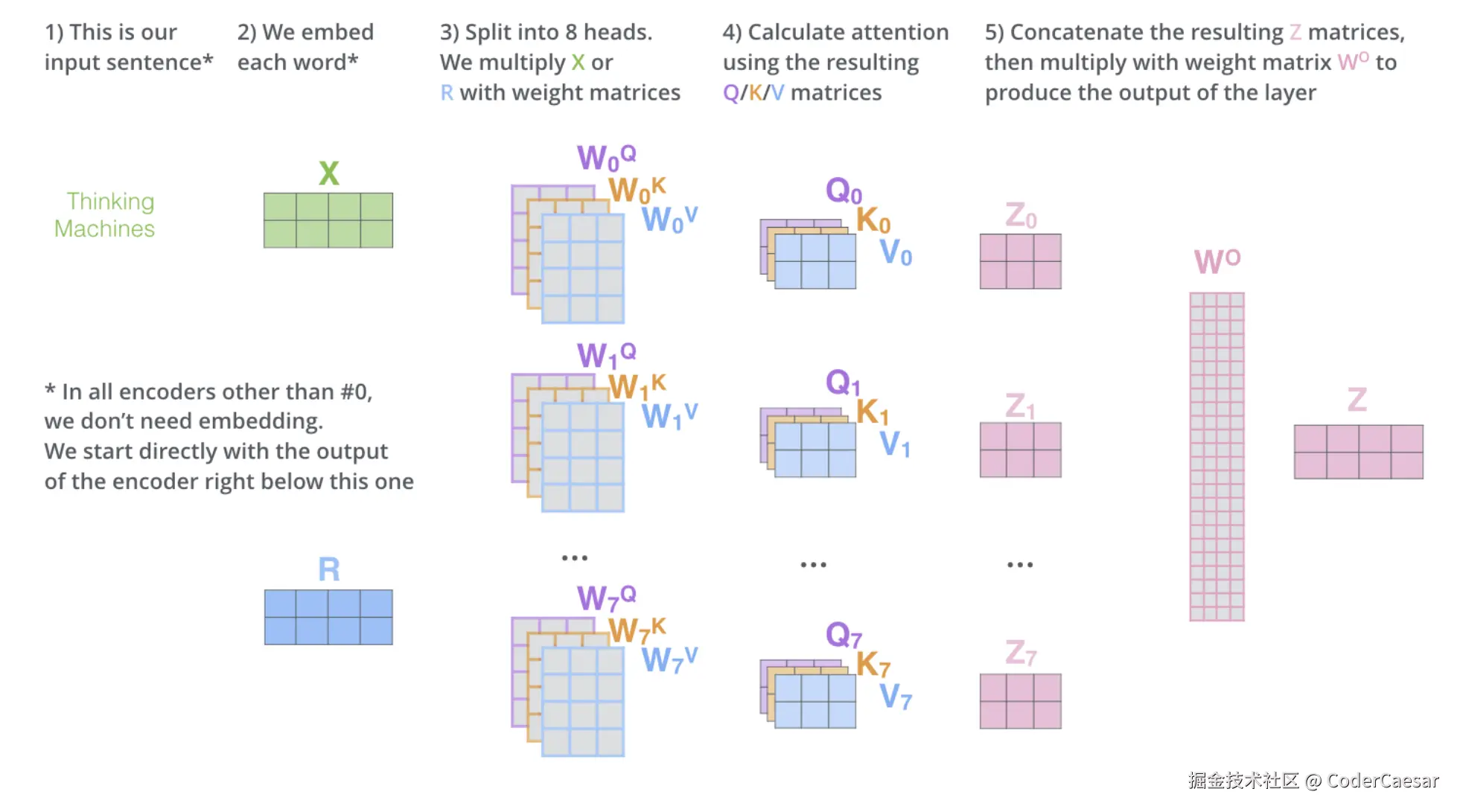
将所有步骤，汇聚成上面一张图。

上图中有个说明：

In all encoders other than #0, we don't need embedding. We start directly with the output of the encoder right below this one.

除了ENCODER#0之外的其他ENCODER（论文中设定了6个ENCODER，还剩下5个），都不需要enbedding操作。我们直接从紧邻其下方的ENCODER的输出开始（ENCODER是从0号往上堆叠的）。用人话说：只有ENCODER#0需要enbedding操作，作为ENCODER#0的输入，其他ENCODER的输入是上一个ENCODER的输出。每一层ENCODER的 attention 层的输出就是上图中的 <math xmlns="http://www.w3.org/1998/Math/MathML"> Z \mathbf{Z} </math>Z。注意每层ENCODER的输出并不是上图的 <math xmlns="http://www.w3.org/1998/Math/MathML"> Z \mathbf{Z} </math>Z，还需要一层 FFNN 计算才是该层ENCODER的输出。

Now that we have touched upon attention heads, let's revisit our example from before to see where the different attention heads are focusing as we encode the word "it" in our example sentence:

既然我们已经提到了多个注意力头，那就回看下我们之前的例子，当我们在 encode 例句中的单词 it 时，看看不同的注意力头分别关注什么地方。

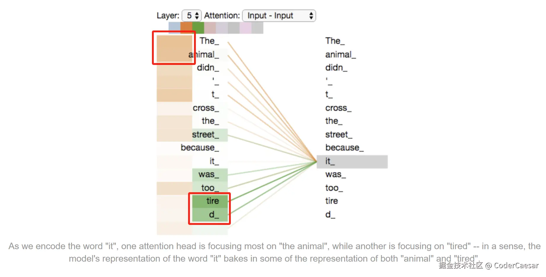
上图中，在第5层，有一个 attention head （棕色）在 encode 单词 it 时，关注到了 "the animal"，而另一个 attention head （绿色）在 encode 单词 it 时，关注到了 "tired"，这样 it 的表示既包含了 animal 的信息又包含了 tired 信息。

更多干货欢迎各位大佬关注wx公众号：double6

参考

The Illustrated Transformer -- Jay Alammar