Interplanetary shocks are one of the crucial dynamic processes in the Heliosphere. They accelerate particles into a high energy, generate plasma waves, and could potentially trigger geomagnetic storms in the terrestrial magnetosphere disturbing significantly our technological infrastructures. In this study, two IP shock events are selected to study the temporal variations of the shock parameters using magnetometer and ion plasma measurements of the STEREO−A and B, the Wind, Cluster fleet, and the ACE spacecraft. The shock normal vectors are determined using the minimum variance analysis (MVA) and the magnetic coplanarity methods (CP).
During the May 07 event, the shock parameters and the shock normal direction are consistent. The shock surface appears to be tilted almost the same degree as the Parker spiral, and the driver could be a CIR. During the April 23 event, the shock parameters do not change significantly except for the shock θBn angle, however, the shape of the IP shock appears to be twisted along the transverse direction to the Sun-Earth line as well. The driver of this rippled shock is SIRs/CIRs as well. Being a fast-reverse shock caused this irregularity in shape.
The solar corona is hotter than the photosphere, the chromosphere, and the transient layers beneath it. As a result, the high temperatures ionize atoms, creating a plasma of free-moving electrons and ions, known as the solar wind. Historically, (Parker, 1958) predicted the existence of the solar wind and coined the term "solar wind". He deducted it based on German astronomer Ludwig Bierman's observation of how the comet tail always points away from the Sun (Biermann, 2013). The existence of the solar wind was confirmed by the Mariner 2 spacecraft (Snyder and Neugebauer, 1965). The solar wind is a collisionless plasma, and it flows at both supersonic and super-Alfvénic speed, meaning they exceed the Alfvén speed, which is the speed of magnetohydrodynamic waves in a plasma. A shock wave is where a fluid changes from supersonic to subsonic speed. Therefore, the fast-moving solar wind tends to create a shock on its journey. Hence, interplanetary (IP) shocks are common through the heliosphere , which is a bubble-like region of space surrounding the Sun and extending far beyond the orbits of the planets and is filled with the solar wind. There are a few varieties of shocks such as planetary bow shocks, shocks that are risen due to the stream interaction regions (SIR), which is called co-rotation interaction region (CIR) when extending beyond 1 AU, and coronal mass ejection (CME) driven shocks. IP shocks are one of the main and efficient accelerators of energetic particles (Tsurutani and Lin, 1985; Keith and Heikkila, 2021). These accelerated particles can cause disturbances to the geomagnetic field and are hazardous to astronauts and satellites. (IP) shocks driven by (CMEs) precede large geomagnetic storms (Gonzalez et al., 1994). Large geomagnetic storms can damage oil and gas pipelines and interfere with electrical power infrastructures. GPS navigation and high-frequency radio communications are also affected by ionosphere changes brought on by geomagnetic storms (Cid et al., 2014) and can cause internet disruptions around the world for many months (Jyothi, 2021). Therefore, IP shocks are important in determining and understanding space weather.
The main goal of this thesis is to study and determine parameters such as IP shock normals, upstream and downstream plasma parameters (magnetic field, density, temperature, velocity), and how they vary in their temporal evolution. There are several methods for determining the shock normal vector (Paschmann and Daly, 1998). In this thesis, the minimum variance analysis (MVA) and the magnetic coplanarity method (CP) are used. These two methods are primarily utilized because they require solely magnetic field data. The data are from NASA's twin Solar Terrestrial Relations Observatory Ahead (STEREO−A) and Behind (STEREO−B) (Kaiser et al., 2008), the Wind (Ogilvie and Desch, 1997), and Advanced Composition Explorer (ACE) spacecraft Stone et al. (1998c), and ESA's four identical Cluster constellation satellites--Cluster-1 (C1), Cluster-2 (C1), Cluster-3 (C3), and Cluster-4 (C4) (Escoubet et al., 1997). The temporal resolution of the magnetometers of the heliospheric (and the Cluster) spacecraft is significantly higher than the plasma instruments because the variations are quite slow in the heliosphere. So, any agreement between the two methods indicates relatively accurate shock normal vectors (Facskó et al., 2008, 2009, 2010). Here, two events are studied, one is May 07, 2007, and the other is April 23. The data selection year, 2007, is special because location-wise it was the year when twin STEREO−A and B spacecraft were closer to the Sun-Earth line until their gradual separation from each other in the following years. Later, the spatial separation is so high that it is hard to distinguish the spatial and temporal changes. Hence, shocks during this period are proper to study shock propagation and their temporal developments in the case of using these spacecraft.
Chapter 2 introduces the basics of plasma physics and magnetohydrodynamics , which are the governing equations of these heliosphere phenomena. Chapter 3 discusses a brief description ofthe Sun, the solar wind, and the interplanetary magnetic field . Chapter 4 is about instrumentation , database , and methods . Chapter 5 presents the results and discusses them. Chapter 6 is the summary and conclusions.
Chapter 2 Basics of Magnetohydrodynamics
▍2.1 Plasma ▍
The term plasma for this state of matter was coined by Irvin Langmuir after its similarity with the blood plasma carrying white and red cells (Tonks, 1967). A plasma is a set of charged particles made up of an equal number of free carriers for positive and negative charges. Having nearly the same number of opposite charges ensures that the plasma appears quasi-neutral from the outside. Free particle carriers mean the particles inside a plasma must have enough kinetic (thermal) energy to overcome the potential energies of their nearest neighbors, which means a plasma is a hot and ionized gas. There are the three basic criteria for a plasma (Baumjohann and Treumann, 2012; Chapters 1-4).
The first criterion is a test-charged particle is clouded by its opposite-charged particles, canceling the electric field of the test particle. This is known as theDebye shielding and its so−called Debye−lenght, λ_D, is defined as follows:
where ϵ_0 is thefree space permittivity , k_B the Boltzmann constant , T_e = T_i the electron and ion temperature , ne the electron plasma density , and e electric charge.
To ensure the quasineutrality of a plasma, the system length L must be greater than the Debye length
The second criterion is since the Debye shielding results from the collective behavior of particles inside the Debye sphere with the radius λ_D, the Debye sphere must contain enough particles
which indicates the mean potential energy of particles between their nearest neighbors must be less than their mean individual energies.
The third criterion is the collision time scale τ of the system is greater than the inverse of the plasma ω⁻¹_p , electron Ω⁻¹_e , and ion Ω⁻¹_i cyclotron gyrofrequencies.
By solving each particle, plasma dynamics can be described, but this approach is too difficult and inefficient. Therefore, there are certain approximations, depending on the corresponding problems. Magnetohydrodynamics is one such approximation that instead of taking account of individual particles, the plasma is assumed as a magnetized fluid.
In this section, the magnetohydrodynamics (MHD) equations are briefly introduced without too much detail and derivations. The following formulizations are based on (Baumjohann and Treumann, 2012)page 138-158, (Murphy, 2014), (Freidberg, 2014) and (Antonsen Jr., 2019). Magnetohydrodynamics (MHD) was developed by Hannes Alfvén (Davidson, 2002). MHD equations are the result of coupling the Navier-Stokes equations (the fluid equations) to the Maxwell equations. In the MHD, the plasma is treated as a single fluid with macroscopic parameters such as average density, temperature, and velocity. Since plasma consists of generally two species of particles, namely electrons, and ions, the different species should be handled together. Hence, the single fluid approximation is utilized.
单流体磁流体力学(MHD)理论体系
本节简要介绍磁流体力学(MHD)方程,不涉及过多细节与推导。以下公式化表述基于以下文献:(Baumjohann and Treumann, 2012)第138-158页、(Murphy, 2014)、(Freidberg, 2014) 和 (Antonsen Jr., 2019)。
By using the single fluid variables, the single fluid MHD equations can be defined as follows:
The continuity equation for the mass density
The momentum equation
where ρe denotes the charge density, and E, B electric and magnetic fields.
The generalized Ohm's law
where η is magnetic diffusivity , and ηJ is the resistive term. Amp`ere's law
where µ_0 is the vacuum magnetic permeability, ϵ_0 is vacuum permittivity.
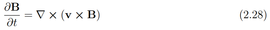
Faraday's law
magnetic field divergence constraint
-- 单流体MHD方程组
使用单流体变量,可定义单流体MHD方程组如下:
质量密度的连续性方程:
动量方程:
其中ρ_e表示电荷密度,E、B分别表示电场和磁场。
广义欧姆定律:
为磁扩散率,ηJ为电阻项。
安培定律:
其中μ_0为真空磁导率,ε_0为真空介电常数。
法拉第定律:
磁场无散约束:
The MHD approximations are valid when the characteristic speed of the system is much slower than the speed of light,
the characteristic frequency, ω, must be smaller than the ion cyclotron frequency ωi
the characteristic scale length L of the system must be longer than the mean free path rgi of ion gyroradius
the characteristic scale times must be larger than the collision times as stated in equation 2.4.
当满足以下条件时,MHD近似成立:
系统特征速度远小于光速,
特征频率ω必须小于离子回旋频率ω_i,
系统特征尺度L必须大于离子回旋半径rgi的平均自由程,
特征时间尺度必须大于如方程2.4所述的碰撞时间。
▍ 2.3 MHD wave modes**▍**
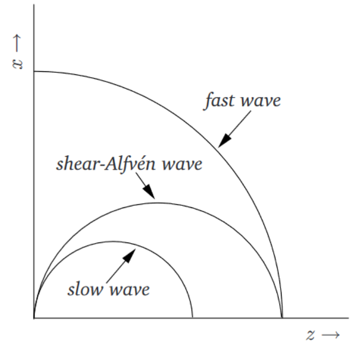
Plasma is considered a highly conductive fluid, which consists of charged particles. Therefore, MHD waves in plasma fundamentally arise from two distinct wave speeds: the sound speed of a fluid and the Alfv´en speed, which is due to the magnetic field pressure and tension. Their combination gives rise to magnetosonic waves. Thus, in MHD there are three wave modes--namely slow magnetosonic, the shear-Alfv´enic and the fast magnetosonic waves (Fitzpatrick, 2014) in addition to the sound wave, as seen in Figure 2.1.
Figure 2.1: Phase velocities of the three MHD waves. (Figure is from Fitzpatrick, 2014; Figure 7.1)
The derivation of the waves can be obtained from the linearized MHD dispersion relation.
sound wave
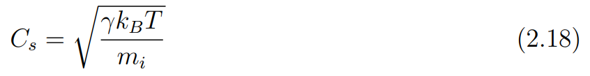
The sound wave is due to a compressible fluid and the wave is longitudinal. The sound speed is defined as:
where γ is the polytropic index and in space plasma , it is in the range 1 < γ < 5/3 (Livadiotis and Nicolaou, 2021), k_B is the Boltzmann constant, T is temperature, mi is mass of a particle species.
Mach number
TheMach number , a ratio of flow to the (thermal) sound speed
Alfvén speed
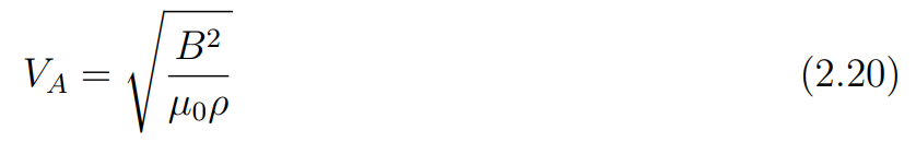
The shear Alfvénwave is incompressible and transverse. The Alfvénspeedis defined as follows:
here B²/μ₀ is the magnetic pressure and ρ is density.
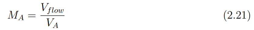
magnetic Mach number
Similarly, the magnetic Mach number , which is defined as a ratio between the flow speed V_f low and the Alfvénic speed V_A, is defined as follows:
magnetosonic waves
The magnetosonic waves are as follows:
where b term is as follows:
声速
波动方程的推导可以从线性化的MHD色散关系中获得。声波源于可压缩流体,是一种纵波。声速定义为:
其中:
γ 是多变指数,在空间等离子体中范围为 1 < γ < 5/3;
k_B 是玻尔兹曼常数;
T 是温度;
m_i 是粒子质量。
马赫数(流动速度与声速之比)
Alfvén 速度
剪切阿尔芬波是不可压缩的横波。阿尔芬速度定义为:
其中:
B²/μ₀ 表示磁压
ρ 是密度
磁马赫数(流动速度与阿尔芬速度之比)
磁声波
其中b项为:
The equation 2.22 has two terms. The term containing (+) is the fast magnetosonic wave while the one containing (-) is the slow magnetosonic wave. When V_A >> V_s or V_s >> V_A in 2.23, as well as the wave propagation direction, is nearly perpendicular to the magnetic field (cos²θ << 1),
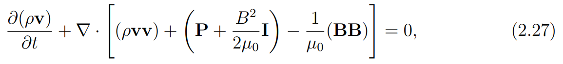
When plasmas of different properties collide, they reach equilibria, resulting in the boundaries separating neighboring plasma regions (Baumjohann and Treumann, 2012; Chapter 8). These boundary regions are called discontinuities, and in astrophysics , heliopause and magnetopauseare examples of these discontinuities. Through discontinuities, the field and plasma parameters change abruptly, but these sudden changes satisfy a few conditions, namely the Rankine-Hugoniot jump conditions. To derive the jump conditions, it is suitable to integrate the conservation laws across the discontinuity. Therefore, it is better to write the single fluid MHD equations 2.2 in conservative form, assuming that the two sides of the discontinuity satisfy an ideal single-fluid MHD. Following some notations and derivations of (Baumjohann and Treumann, 2012; Chapter 8), the ideal single-fluid MHD equations in conservative forms are defined below:
where P the plasma pressure, B the magnetic field magnitude,B the magnetic field vector, µ0 the vacuum permeability, and I the identity tensor.
where for slowly variable fields µ0j = ∇ × B and the ideal Ohm's law E = −∇ ×B are implemented as well as neglecting charges ρE = 0, and w = c_v*P/ρ*k_B is the internal enthalpy. For completion, the equation of state is set:
where p is the scalar pressure.
Choosing a co-moving reference frame with discontinuity, a steady-state situation is assumed that all the time-dependent terms are canceled, leaving the flux terms in the conservation laws.
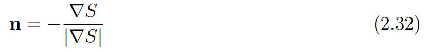
A discontinuity causes the plasma parallel to the discontinuity to stay the same while the plasma perpendicular to the discontinuity changes. For these reasons, a two-dimensional function S(x)=0 can be used to characterize the discontinuity surface, and the normal vector to the discontinuity, n, is defined as follows
To the direction of the n the vector derivative has only one component ∇ = n( ∂/∂n). After these considerations, integrating over the discontinuity for the flux terms has to be done.
磁感应方程:
磁场散度方程:
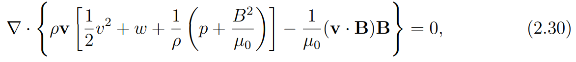
能量守恒方程:
其中对于缓变场,采用μ₀j = ∇ × B 和理想欧姆定律 E = -∇ × B ,并忽略电荷项 ρE = 0,w = c_v*P/ρ*k_B表示内焓。为完整起见,状态方程设为:
Remembering only two perpendicular sides of the discontinuity contribute twice to the integration, a quantity X crossing S becomes
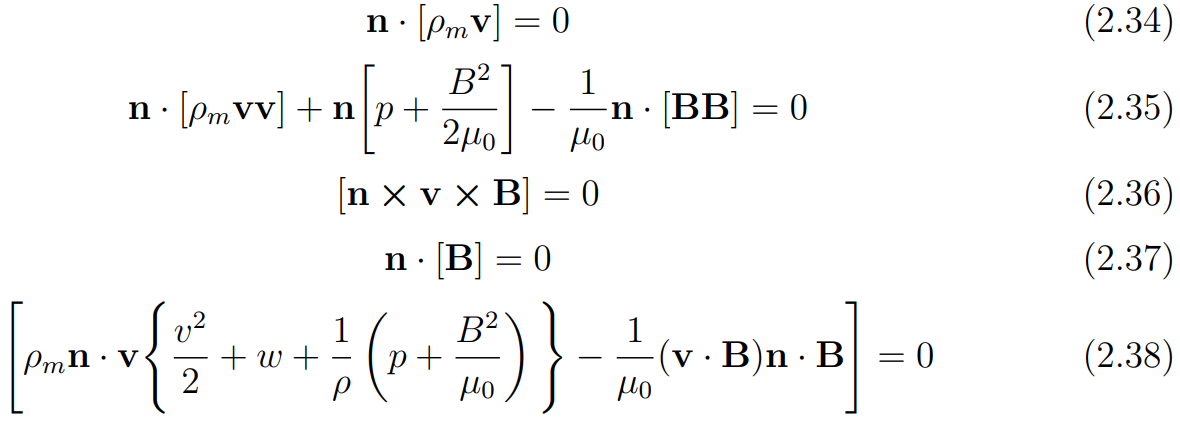
where parenthesis X indicates the jump of a quantity X. Now replacing the conservation laws of the ideal one-fluid MHD with the jump conditions, the Rankine-Hugoniot conditions are defined as follows:
From the equations above, the normal component of the magnetic field is continuous across all discontinuities, which leads to its jump condition vanishing.
Also normal direction mass flow is continuous:
Splitting the fields between the normal and tangential components, the remaining jump conditions are derived:
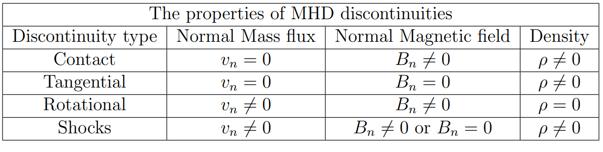
where subscript t and n denote normal and tangential components respectively. The equations 2.39 and 2.40 demonstrate that the normal components of the magnetic field, as well as the mass flow, are constant across the discontinuity. The Rankine-Hugoniot conditions provide the four types of MHD discontinuities (Baumjohann and Treumann, 2012; Chapter-8), namely contact discontinuity, tangential discontinuity, rotational discontinuity, and shocks as the values are defined in Table 2.1.
Table 2.1: Some properties of MHD discontinuities. (The values are from Oliveira, 2015)
Contact discontinuity
Contact discontinuity is determined by the condition when there is no normal mass flow across discontinuities, which means from the Rankine-Hugoniot conditions v_n = 0. When B_n ̸= 0 or B_n = 0, the only quantity that experiences a change across the discontinuity is the density, ρ ̸= 0. Due to these constraints, the plasma on the two sides of the discontinuity are attached and connected by the normal component of the magnetic field, As a result, they flow together at the same tangential speed. This is known as the contact discontinuity.
Tangential discontinuity is when B_n = 0 in addition to v_n = 0, only non-trivially satisfied jump condition is the total pressure balance in the equation 2.41, which indicates that a discontinuity is created between two plasma with total pressure balance on both sides and no mass and magnetic fluxes are crossing across the discontinuity while all other quantities are changing. This is the tangential discontinuity.
Rotational discontinuity is formed when there is a continuous normal flow velocity v_n = 0 with a non-vanishing B_n ̸= 0 such that from the equations 2.42 and 2.43 the tangential velocity and the magnetic field can only change together , especially the equation 2.43 indicates they rotate together when crossing the discontinuity. Shocks Unlike the previous three discontinuities, shocks are irreversible in that the entropy increases (Goedbloed et al., 2019). And one of the main distinctive characteristics of shocks is normal fluxes of the Rankine-Hugionot conditions take non-zero values, ρv_n ̸= 0, and the density ρ is discontinuous.
Consequently of the three wave modes, there are corresponding three shocks -- fast shock (FS), intermediate shock (IS), and slow shock (SS) (Tsurutani et al., 2011). When the fast wave speed is greater than the upstream magnetosonic speed 2.25, the fast shocks (FSs) are formed. Similarly, when the shear-Alfv´en wave speed is greater than the upstream Alfv´en velocity 2.20, the intermediate shocks (ISs) are formed, and when the slow wave speed is greater than the upstream (thermal) sound speed 2.18, the slow shocks (SSs) are formed with their respective Mach numbers greater than at least 1.
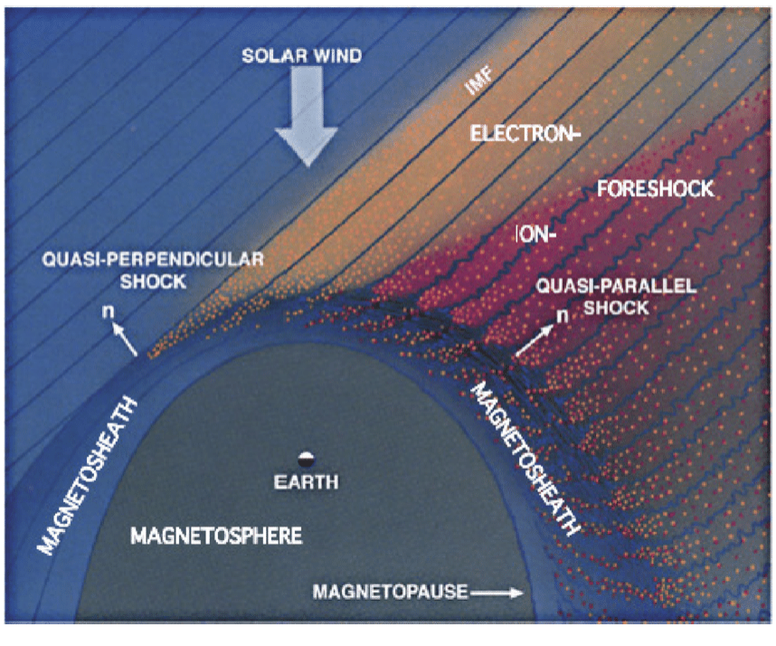
The three MHD waves 2.3 are anisotropic, which means their speeds depend on the angle between wave propagation direction and the upstream (unshocked) magnetic field. An illustration of this is the Parker spiral propagation of the solar wind such that the interplanetary magnetic field (IMF) hits, for example, the Earth from the morning side, it creates parallel and perpendicular shocks concerning the shock normal and the upstream magnetic field B as shown in Figure 2.2.
Figure 2.2: The solar wind interaction with the Earth's bow shock.(Figure is from Oliveira, 2015; Figure 2-5)