人工智能概述
人工智能分为:符号学习,机器学习。
机器学习是实现人工智能的一种方法,深度学习是实现机器学习的一种技术。
机器学习:使用算法来解析数据,从中学习,然后对真实世界中是事务进行决策和预测。如垃圾邮件检测,楼房价格预测。
深度学习:模仿人类神经网络,建立模型,进行数据分析。如,人脸识别,语义理解,无人驾驶。
工具
Anaconda
Anaconda是一个方便的python包管理和环境管理的软件
可以跨平台,多python版本并存,部署方便
Jupyter Notebook
Jupyter notebook是一个开源的web应用程序,允许开发者方便的创建和共享代码文档
允许吧代码写入独立的cell中,单独执行。用户可以单独测试特定代码块,无需从头开始执行代码。
基础工具包
Panda
强大的分析结构化数据的工具集,可用于快速实现数据导入/出,索引
Numpy
使用Python进行科学计算的基础软件包。核心:基于N维数组对象ndarray的数组运算。
Matplolib
Python基础绘图库,几行代码即可生成绘图
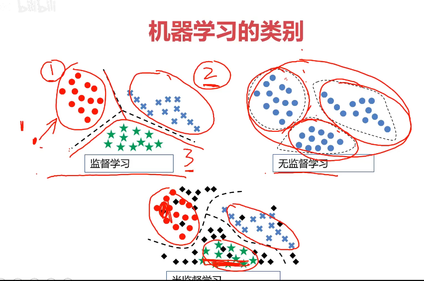
机器学习的类别
监督学习(Supervised Learning)
-训练数据包括正确的结果
无监督学习(Unsupervised Learning)
-训练数据不包括正确的结果
半监督学习(Semi-supervised Learning)
-训练数据包括少量正确的结果
强化学习(Reinforcement Learning)
-根据每次结果收获的奖惩进行学习,实现优化
监督学习:线性回归,逻辑回归,决策树,神经网络,卷积神经网络,循环神经网络。
无监督学习:聚类算法
混合学习:监督学习+无监督学习
什么是回归分析?
回归分析:根据数据,确定两种或两种以上变量间相互依赖的定量关系
线性回归:回归分析中,变量与因变量存在线性关系
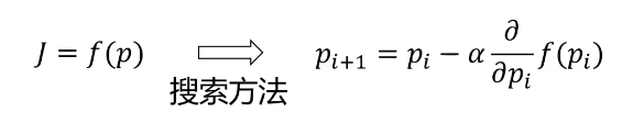
梯度下降法:
寻找极小值的一种方法。通过向函数上当前点对应梯度的反方向的规定步长距离点进行迭代搜索,直到在极小点收敛。
Scikit-learn
Python语言中专门针对机器学习应用而发展起来的一款开源框架(算法库),可以实现数据预处理,分类,回归,降维,模型选择等常用的机器学习算法
集成了机器学习中各类成熟的算法,不支持深度学习和强化学习。
https://scikit-learn.org/stable/index.html
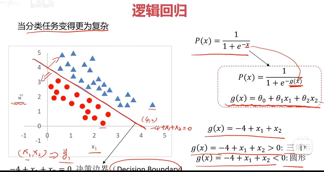
分类问题
分类:根据已知样本的某些特征,判断一个显得样本属于那种已知的样本类
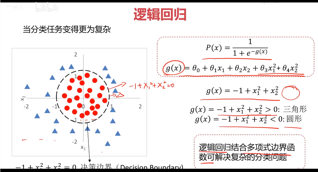
使用逻辑回归拟合数据,可以很好的完成分类任务
线性:y=ax+b
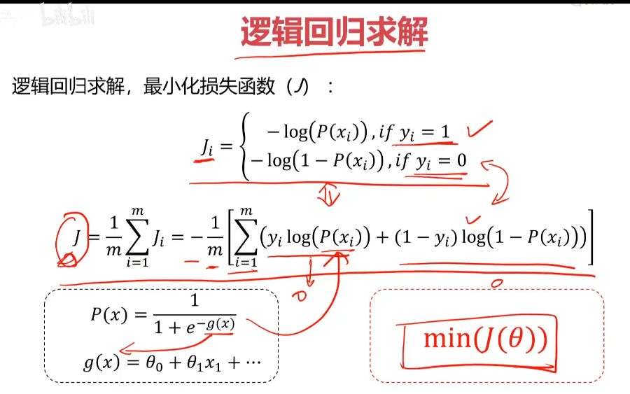
逻辑:y=1/(1+e^(-x)) sigmoid方程 通用公式:P(x)=1/(1+e^(-g(x)))
找到决策边界(Decision Boundary)很关键
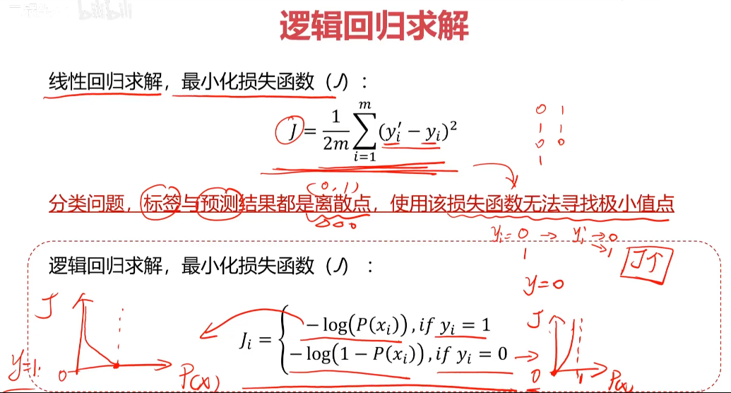
分类任务的损失函数:
逻辑回归实战
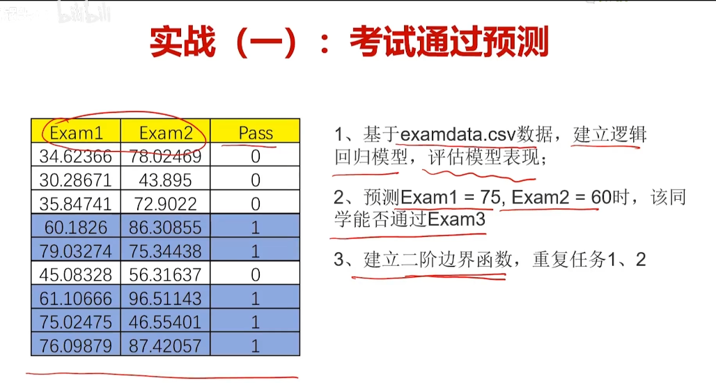
实战1考试通过预测
无监督学习
机器学习的一种方法,没有给定先标记过的训练示例,自动对输入的数据进行分类或分群
聚类分析
聚类分析又称为群分析,根据对象某些属性的相似度,将其自动划分为不同的类别。
应用场景:客户划分,基因聚类,新闻关联
KMeans
K-均值算法:以空间中k个点为中心进行聚类,对最靠近他们的对象归类,是聚类算法中最为基础但也最为重要的算法。
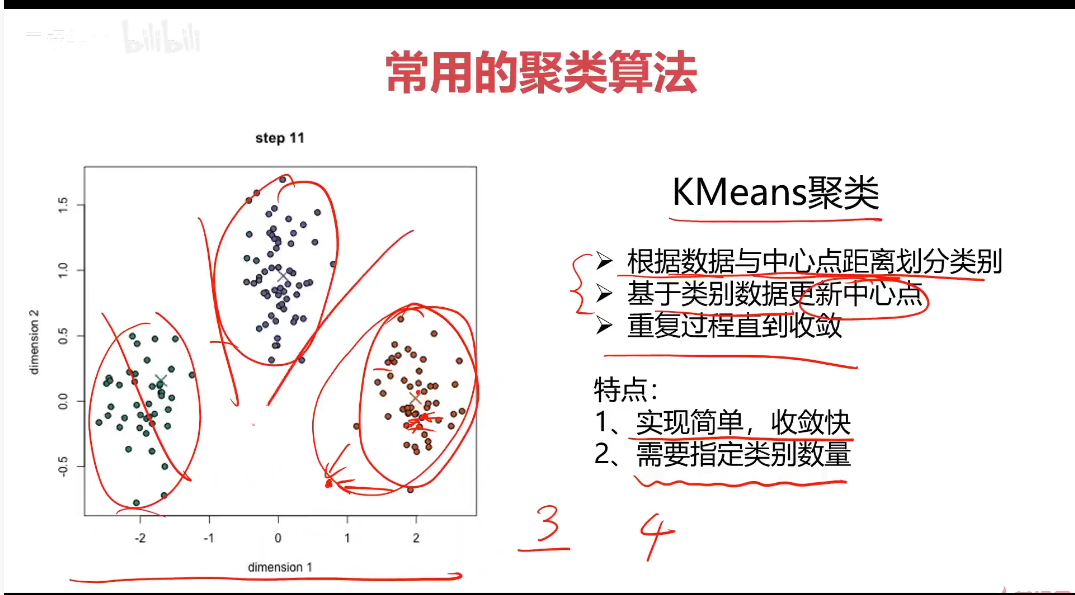
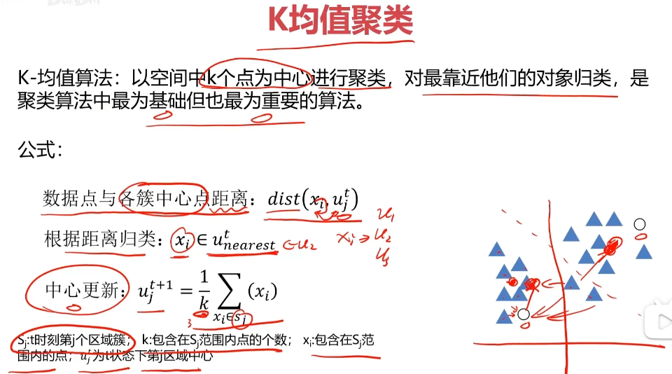
算法流程:
1.选择聚类的个数k
2.确定聚类的中心
3.根据点道聚类中心聚类确定各个点所属类别
4.根据各个类别数据更新聚类中心
5.重复以上步骤直到收敛(中心点不再变化)
优点:
1.简单易实现,收敛速度快
2.参数少
缺点:
1.必须设置簇的数量
2.随机选择初始聚类中心,结果可能缺乏一致性
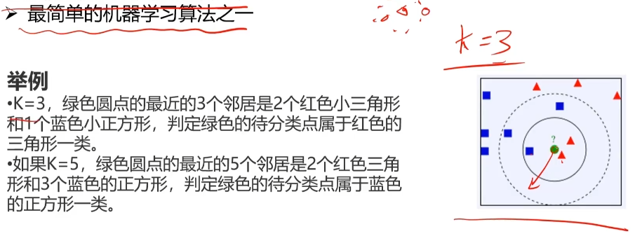
KNN
K近邻分类模型
给定一个训练数据集,对新的输入实例,在训练数据集中找到与该实例最邻近的K个实例(也就是上面所说的K个邻居),这K个实例的多数属于某个类,就把该输入实例分类到这个类中
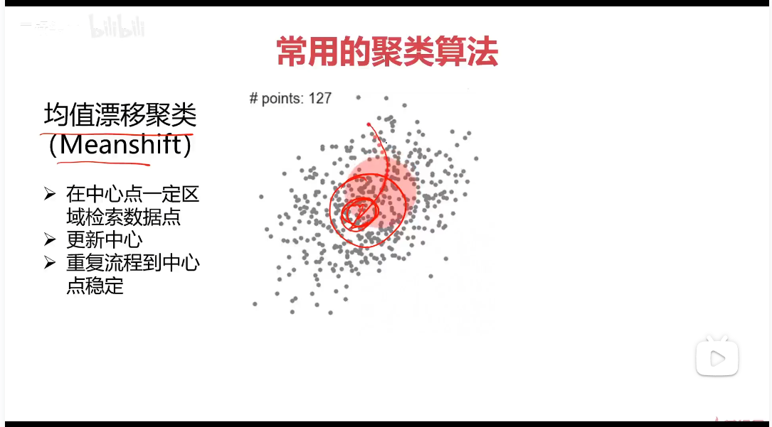
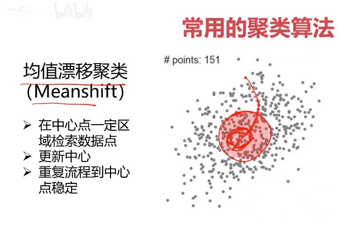
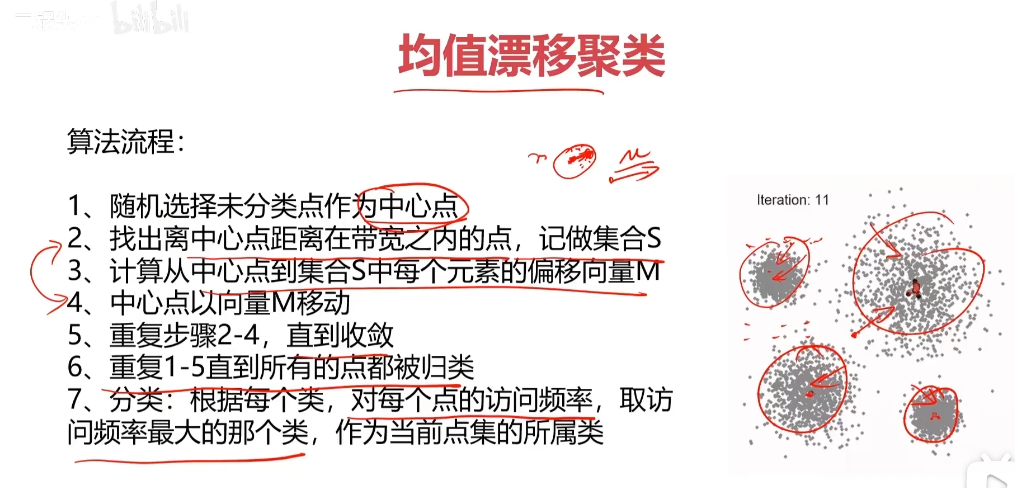
Mean-shift
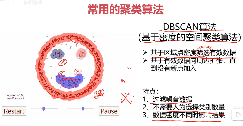
聚类实战
KMeans实现聚类
模型训练
python
form sklearn.cluster import KMeans
KM = KMeans(n_clusters=3,random_state=0)
KM.fit(X)
获取中心点:
python
centers = KM.cluster_centers_准确率计算:
python
form sklearn.metrics import accuracy_score
accuracy = accuracy_score(y,y_predict)
预测结果矫正(比如原始数据是0,1,2但是KNN预测的乱序了,如2,0,1):
python
y_cal = []
for i in y_predict:
	if i == 0:
		y_cla.append(2)
	elif i == 1:
		y_cal.append(0)
	else:
		y_cal.append(1)
	print(y_predict, y_cal0
Meanshift实现聚类
python
自动计算带宽(区域半径)
from sklearn.cluster import MeanShift,estimate_bandwidth
#detect bandwidth
bandwidth = estimate_bandwidth(X,n_samples=500)
#X样本数量,n_samples采样的样本数量
模型建立于训练
ms = MeanShift(bandwidth=bandwidth)
ms.fit(X)
KNN实现分类
模型训练
python
form sklearn.neighbors import KNeighborsClassifier
KNN = KNeighborsClassifier(n_neighbors=3)
KNN.fit(X,y)
实战:2D数据类别划分
1.采用Kmeans算法实现2D数据自动聚类,预测V1=80,V2=60数据类别;
2.计算预测准确率,完成结果矫正
3.采用KNN,Meanshift算法,重复步骤1-2
KMeans算法实现
python
#load the data
import pandas as pd
import numpy as np
data = pd.read_csv('data.csv')
data.head()
python
#define X and y
X = data.drop(['labels'],axis=1)
y = data.loc[:,'labels']
y.head()
python
pd.value_counts(y)
python
%matplotlib inline
from matplotlib import pyplot as plt
plt.scatter(X.loc[:,'V1'],X.loc[:'V2'])
plt.title("un-labled data")
plt.xlabel('V1')
plt.ylabel('V2')
plt.show()

fig1 = plt.figure()
label0 = plt.scatter(X.loc[:,'V1'][y==0],X.loc[:'V2'][y==0])
label1 = plt.scatter(X.loc[:,'V1'][y==1],X.loc[:'V2'][y==1])
label2 = plt.scatter(X.loc[:,'V1'][y==2],X.loc[:'V2'][y==2])

plt.title("labled data")
plt.xlabel('V1')
plt.ylabel('V2')
plt.legend((label0,label1,label2),('label0','label1','label2'))
plt.show()
python
print(X.shape, y.shape)
python
#set the model
from sklearn.cluster import KMeans
KM = KMeans(n_cluster=3,random_sate=0)
KM.fit(X)

centers = KM.cluster_centers_
fig3 = plt.figure()
label0 = plt.scatter(X.loc[:,'V1'][y==0],X.loc[:'V2'][y==0])
label1 = plt.scatter(X.loc[:,'V1'][y==1],X.loc[:'V2'][y==1])
label2 = plt.scatter(X.loc[:,'V1'][y==2],X.loc[:'V2'][y==2])

plt.title("labled data")
plt.xlabel('V1')
plt.ylabel('V2')
plt.legend((label0,label1,label2),('label0','label1','label2'))
plt.scatter(centers[:,0],centers[:,1])
plt.show()
python
#test data: V1=80,V2=60
y_predict_test = KM.predict([[80, 60]])
print(y_predict_test )

#predict based on training data
y_predict = KM.predict(X)
print(pd.value_counts(y_predict), pd.value_counts(y))

from sklearn.metrics import accuracy_score
accuracy = accuracy_score(y,y_predict)
print(accuracy)
python
#visualize the data and results
fig4 = plt.subplot(121)
label0 = plt.scatter(X.loc[:,'V1'][y_predict==0],X.loc[:'V2'][y_predict==0])
label1 = plt.scatter(X.loc[:,'V1'][y_predict==1],X.loc[:'V2'][y_predict==1])
label2 = plt.scatter(X.loc[:,'V1'][y_predict==2],X.loc[:'V2'][y_predict==2])

plt.title("predict data")
plt.xlabel('V1')
plt.ylabel('V2')
plt.legend((label0,label1,label2),('label0','label1','label2'))
plt.scatter(centers[:,0],centers[:,1])

fig5 = plt.subplot(122)
label0 = plt.scatter(X.loc[:,'V1'][y==0],X.loc[:'V2'][y==0])
label1 = plt.scatter(X.loc[:,'V1'][y==1],X.loc[:'V2'][y==1])
label2 = plt.scatter(X.loc[:,'V1'][y==2],X.loc[:'V2'][y==2])

plt.title("labled data")
plt.xlabel('V1')
plt.ylabel('V2')
plt.legend((label0,label1,label2),('label0','label1','label2'))
plt.scatter(centers[:,0],centers[:,1])

plt.show()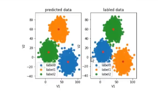
python
 #correct the results
 y_corrected = []
 for i in y_predict:
 		if i == 0:
 			y_corrected.append(1)
 		elif i == 1:
  			y_corrected.append(2)
  		else:
  			y_corrected.append(0)
 print(pd.value_counts(y_corrected), pd.value_counts(y))
python
print(accuracy_score(y, y_corrected))
python
y_corrected = np.array(y_corrected)
print(type(y_corrected))
#visualize the data and results
fig6 = plt.subplot(121)
label0 = plt.scatter(X.loc[:,'V1'][y_corrected==0],X.loc[:'V2'][y_corrected==0])
label1 = plt.scatter(X.loc[:,'V1'][y_corrected==1],X.loc[:'V2'][y_corrected==1])
label2 = plt.scatter(X.loc[:,'V1'][y_corrected==2],X.loc[:'V2'][y_corrected==2])

plt.title("predict data")
plt.xlabel('V1')
plt.ylabel('V2')
plt.legend((label0,label1,label2),('label0','label1','label2'))
plt.scatter(centers[:,0],centers[:,1])

fig7 = plt.subplot(122)
label0 = plt.scatter(X.loc[:,'V1'][y==0],X.loc[:'V2'][y==0])
label1 = plt.scatter(X.loc[:,'V1'][y==1],X.loc[:'V2'][y==1])
label2 = plt.scatter(X.loc[:,'V1'][y==2],X.loc[:'V2'][y==2])

plt.title("labled data")
plt.xlabel('V1')
plt.ylabel('V2')
plt.legend((label0,label1,label2),('label0','label1','label2'))
plt.scatter(centers[:,0],centers[:,1])

plt.show()
KNN算法实现
查看数据
python
X.head()
y.head()
python
#establish a KNN model
from sklearn.neighbors import KNeighborsClassifier
KNN = KNeighborsClassifier(n_neighbors=3)
KNN.fit(X,y)
python
#predict based on the test data V1=80, V2=60
y_predict_knn_test = KNN.predict([[80, 60]])
y_predict_knn = KNN.predict(X)
print(y_predict_knn_test)
print('knn accuracy:', accuracy_score(y, y_predict_knn))
python
fig6 = plt.subplot(121)
label0 = plt.scatter(X.loc[:,'V1'][y_predict_knn==0],X.loc[:'V2'][y_predict_knn==0])
label1 = plt.scatter(X.loc[:,'V1'][y_predict_knn==1],X.loc[:'V2'][y_predict_knn==1])
label2 = plt.scatter(X.loc[:,'V1'][y_predict_knn==2],X.loc[:'V2'][y_predict_knn==2])

plt.title("knn results")
plt.xlabel('V1')
plt.ylabel('V2')
plt.legend((label0,label1,label2),('label0','label1','label2'))
plt.scatter(centers[:,0],centers[:,1])

fig7 = plt.subplot(122)
label0 = plt.scatter(X.loc[:,'V1'][y==0],X.loc[:'V2'][y==0])
label1 = plt.scatter(X.loc[:,'V1'][y==1],X.loc[:'V2'][y==1])
label2 = plt.scatter(X.loc[:,'V1'][y==2],X.loc[:'V2'][y==2])

plt.title("labled data")
plt.xlabel('V1')
plt.ylabel('V2')
plt.legend((label0,label1,label2),('label0','label1','label2'))
plt.scatter(centers[:,0],centers[:,1])

plt.show()
MeanShift
python
#meanshift
form sklearn.cluster import MeanShift,estimate_bandwidth
#obtain the bandwidth
bw = estimate_bandwidth(X,n_samples=500)
print(bw)
python
#establish the meanshift model-un-supervised model
ms = MeanShift(bandwidth=bw)
ms.fit(X)
python
y_predict_ms = ms.predict(X)
print(pd.value_counts(y_predict_ms), pd.value_counts(y))
python
fig6 = plt.subplot(121)
label0 = plt.scatter(X.loc[:,'V1'][y_predict_knn_ms==0],X.loc[:'V2'][y_predict_knn_ms==0])
label1 = plt.scatter(X.loc[:,'V1'][y_predict_knn_ms==1],X.loc[:'V2'][y_predict_knn_ms==1])
label2 = plt.scatter(X.loc[:,'V1'][y_predict_knn_ms==2],X.loc[:'V2'][y_predict_knn_ms==2])

plt.title("kmeanshift results")
plt.xlabel('V1')
plt.ylabel('V2')
plt.legend((label0,label1,label2),('label0','label1','label2'))
plt.scatter(centers[:,0],centers[:,1])

fig7 = plt.subplot(122)
label0 = plt.scatter(X.loc[:,'V1'][y==0],X.loc[:'V2'][y==0])
label1 = plt.scatter(X.loc[:,'V1'][y==1],X.loc[:'V2'][y==1])
label2 = plt.scatter(X.loc[:,'V1'][y==2],X.loc[:'V2'][y==2])

plt.title("labled data")
plt.xlabel('V1')
plt.ylabel('V2')
plt.legend((label0,label1,label2),('label0','label1','label2'))
plt.scatter(centers[:,0],centers[:,1])

plt.show()
python
 #correct the results
 y_corrected_ms = []
 for i in y_predict_ms:
 		if i == 0:
 			y_corrected_ms .append(2)
 		elif i == 1:
  			y_corrected_ms .append(1)
  		else:
  			y_corrected_ms .append(0)
 print(pd.value_counts(y_corrected_ms), pd.value_counts(y))
python
#convert the results to numpy array
y_corrected = np.array(y_corrected_ms)
print(type(y_corrected_ms)
python
fig6 = plt.subplot(121)
label0 = plt.scatter(X.loc[:,'V1'][y_predict_knn_ms==0],X.loc[:'V2'][y_predict_knn_ms==0])
label1 = plt.scatter(X.loc[:,'V1'][y_predict_knn_ms==1],X.loc[:'V2'][y_predict_knn_ms==1])
label2 = plt.scatter(X.loc[:,'V1'][y_predict_knn_ms==2],X.loc[:'V2'][y_predict_knn_ms==2])

plt.title("ms correct results")
plt.xlabel('V1')
plt.ylabel('V2')
plt.legend((label0,label1,label2),('label0','label1','label2'))
plt.scatter(centers[:,0],centers[:,1])

fig7 = plt.subplot(122)
label0 = plt.scatter(X.loc[:,'V1'][y==0],X.loc[:'V2'][y==0])
label1 = plt.scatter(X.loc[:,'V1'][y==1],X.loc[:'V2'][y==1])
label2 = plt.scatter(X.loc[:,'V1'][y==2],X.loc[:'V2'][y==2])

plt.title("labled data")
plt.xlabel('V1')
plt.ylabel('V2')
plt.legend((label0,label1,label2),('label0','label1','label2'))
plt.scatter(centers[:,0],centers[:,1])
plt.show()
##总结
kmeans\knn\meanshift
kmeans\meanshift: un-supervised, training data: X; kmeans: category number; meanshift: calculate the bandwidth
knn: supervised; training data: X\y