一、伪谱法
伪谱法作为最优控制领域的经典算法,其基本原理这里不做基本介绍,主要讲解代码实现部分,由于CasADi库本身不自带生成LGL节点和微分矩阵的函数,因此我们首先定义PseudoSpectral对象,包括生成LGL节点和微分矩阵函数的方法。
python
import numpy as np
from numpy.polynomial import legendre as L
from scipy.special import legendre
class PseudoSpectral:
    """
    伪谱法类,基于Legendre-Gauss-Lobatto配点
    """

    def __init__(self, N, tau_interval=[0, 1]):
        """
        初始化伪谱法对象

        参数:
        N: int, 多项式阶数
        tau_interval: list, 时间区间 [t0, tf]
        """
        self.N = N  # 多项式阶数
        self.tau_interval = tau_interval

        # 计算LGL节点和权重(标准区间[-1,1]上)
        self.xi = self._find_LGL_points()  # 标准区间上的配点
        self.omega = self._get_LGL_weights()  # 标准区间上的权重

        # 变换到实际时间区间
        self.tau = self._transform_to_tau(self.xi)  # 实际时间区间上的配点
        self.weights = self._transform_weights(self.omega)  # 实际时间区间上的权重

        # 计算微分矩阵
        self.D = self._get_differentiation_matrix()

        # 计算基函数
        self.basis = self._compute_basis_functions()

    def _get_legendre_coeffs(self, n):
        """获取n阶Legendre多项式的系数"""
        if n == 0:
            return np.array([1])
        elif n == 1:
            return np.array([1, 0])
        else:
            p_prev = np.poly1d([1])
            p_curr = np.poly1d([1, 0])

            for k in range(2, n + 1):
                p_next = ((2 * k - 1) * np.polymul([1, 0], p_curr) - (k - 1) * p_prev) / k
                p_prev = p_curr
                p_curr = p_next

            return p_curr.coefficients

    def _find_LGL_points(self):
        """计算LGL节点"""
        if self.N < 2:
            return np.array([-1, 1])

        coefs = self._get_legendre_coeffs(self.N)
        P = np.poly1d(coefs)
        dP = P.deriv()

        roots = np.roots(dP)
        roots = np.real(roots[np.abs(np.imag(roots)) < 1e-15])
        roots = roots[np.abs(roots) <= 1]

        nodes = np.concatenate(([-1], roots, [1]))
        return np.sort(nodes)

    def _get_LGL_weights(self):
        """计算LGL权重"""
        if self.N < 2:
            return np.array([1, 1])

        x = self.xi
        P = np.poly1d(self._get_legendre_coeffs(self.N))

        w = np.zeros_like(x)
        for i in range(len(x)):
            w[i] = 2 / (self.N * (self.N + 1) * (P(x[i])) ** 2)

        return w

    def _transform_to_tau(self, xi):
        """将标准区间[-1,1]的点变换到实际时间区间"""
        t0, tf = self.tau_interval
        return ((tf - t0) * xi + (tf + t0)) / 2

    def _transform_weights(self, omega):
        """变换权重到实际时间区间"""
        t0, tf = self.tau_interval
        return omega * (tf - t0) / 2

    def _get_differentiation_matrix(self):

        N = self.N
        D = np.zeros((N + 1, N + 1))
        xi = self.xi  # LGL节点

        # 获取N阶Legendre多项式
        P_N = np.poly1d(self._get_legendre_coeffs(N))

        # 计算每个节点上的Legendre多项式值

        D[0, 0] = -N * (N + 1) / 4
        D[N, N] = N * (N + 1) / 4

        # 对角元素 (除端点外) - 按照MATLAB版本处理
        for i in range(1, N):  # 对应MATLAB的2:N
            D[i, i] = 0

        # 非对角元素
        for i in range(N + 1):
            for j in range(N + 1):
                if i != j:
                    D[i, j] = legendre(N)(xi[i]) / (legendre(N)(xi[j]) * (xi[i] - xi[j]))


        return D

    def _compute_basis_functions(self):
        """计算基函数"""
        n = self.N
        basis = np.zeros((n + 1, n + 1))
        x = self.xi

        for i in range(n + 1):
            # 构造拉格朗日基函数
            p = 1
            for j in range(n + 1):
                if i != j:
                    p = np.polymul(p, [1 / (x[i] - x[j]), -x[j] / (x[i] - x[j])])
            basis[:, i] = np.polyval(p, x)

        return basis

    def interpolate(self, y, tau_new):
        """
        在给定点上进行插值

        参数:
        y: 节点上的函数值
        tau_new: 需要插值的点
        """
        # 将tau_new变换回标准区间
        t0, tf = self.tau_interval
        xi_new = 2 * (tau_new - t0) / (tf - t0) - 1

        # 计算插值结果
        result = np.zeros_like(xi_new)
        for i in range(self.N + 1):
            # 构造拉格朗日基函数
            p = 1
            for j in range(self.N + 1):
                if i != j:
                    p = np.polymul(p, [1 / (self.xi[i] - self.xi[j]),
                                       -self.xi[j] / (self.xi[i] - self.xi[j])])
            result += y[i] * np.polyval(p, xi_new)

        return result

    def integrate(self, f):
        """
        使用LGL求积计算函数的积分

        参数:
        f: 节点上的函数值
        """
        return np.sum(self.weights * f)

    def differentiate(self, f):
        """
        计算函数在节点上的导数值

        参数:
        f: 节点上的函数值
        """
        return np.dot(self.D, f)


    def verify_sine_derivative(self):

        t = self.tau

        # 2. 计算原函数在LGL节点上的值
        y1 = np.sin(t)*2/(self.tau_interval[1]-self.tau_interval[0])
        # 3. 用微分矩阵计算导数 (需要考虑时间变换)
        dy1_numerical = self.D @ y1
        dy1_analytical = np.cos(t)        # 5. 打印比较结果
        print('s')

# 运行测试
if __name__ == "__main__":
    N = 5
    t0, tf =0, 1
    ps = PseudoSpectral(N, [t0, tf])
    # 验证导数
ps.verify_sine_derivative()现在结合一个具体的例子,使用伪谱法的应用过程。假设初始状态为,状态转移方程为
状态约束:
控制约束:
指标函数为:
根据伪谱法,假设我们取20阶LGL节点,那么对应42个状态变量,21个控制变量,根据重要的动力学约束,构建等式约束。
因此得到等式约束
整个问题的优化变量,得到微分矩阵
第一个动力学约束为
依次类推得到42个等式的动力学约束,加上初始的2个边界约束,一共44个等式约束
现在根据指标的计算
结合Python的CasADi库来求解,代码如下图
python
# optimal_control.py
from PseudoSpectral import PseudoSpectral
import casadi as ca
import numpy as np
import matplotlib.pyplot as plt
class OptimalControl:
def __init__(self, N=6):
"""
初始化最优控制问题求解器
参数:
N: int, LGL配点阶数
"""
self.ps = PseudoSpectral(N, [-1, 1]) # 使用标准区间
self.N = N
# 时间区间
self.T = 10.0 # 终端时间
# 获取LGL节点和权重
self.tau = self.ps.xi # 配点(标准区间)
self.weights = self.ps.omega # 权重
self.D = self.ps.D # 微分矩阵
def solve(self):
"""求解最优控制问题"""
# 声明状态和控制变量
x1 = ca.SX.sym('x1')
x2 = ca.SX.sym('x2')
x = ca.vertcat(x1, x2)
u = ca.SX.sym('u')
# 系统动力学
xdot = ca.vertcat((1 - x2 ** 2) * x1 - x2 + u, x1)
f = ca.Function('f', [x, u], [xdot], ['x', 'u'], ['xdot'])
# 目标函数
L = x1 ** 2 + x2 ** 2 + u ** 2
L_fun = ca.Function('L', [x1, x2, u], [L])
# 创建连续时间动力学函数
f = ca.Function('f', [x, u], [xdot, L], ['x', 'u'], ['xdot', 'L'])
# 构建NLP问题
# 决策变量
X = ca.SX.sym('X', 2, self.N + 1) # 状态变量在所有节点上的值
U = ca.SX.sym('U', self.N + 1) # 控制变量在所有节点上的值
# 将决策变量转换为向量
w = ca.vertcat(ca.reshape(X, -1, 1), U)
# 目标函数
J = 0
for i in range(self.N + 1):
J += self.weights[i] * L_fun(X[0,i], X[1,i], U[i]) * self.T/2
# 约束
g = []
# 动力学约束
for i in range(2): # 对每个状态分量
# 使用微分矩阵计算数值导数: dx/dtau = D*x
dx_numerical = ca.mtimes(self.D, X[i, :].T)
# 在每个节点上比较数值导数和模型导数
for k in range(self.N + 1):
x_current = [X[0, k], X[1, k]]
u_current = U[k]
# 计算模型动力学 (注意时间变换)
dx_model = f(x=ca.vertcat(x_current[0], x_current[1]),
u=u_current)['xdot'][i] * self.T / 2 # 时间变换系数
# 动力学约束:数值导数 = 模型导数
g.append(dx_numerical[k] - dx_model)
# 边界条件
g.append(X[0, 0] - 0) # x1(0) = 0
g.append(X[1, 0] - 1) # x2(0) = 1
# 构建NLP
nlp = {'x': w, 'f': J, 'g': ca.vertcat(*g)}
# 设置求解器选项
opts = {'ipopt.print_level': 5, 'print_time': 1}
solver = ca.nlpsol('solver', 'ipopt', nlp, opts)
# 设置初值和约束边界
w0 = self._generate_initial_guess()
lbw = -np.inf * np.ones(w.shape[0]) # 决策变量下界
ubw = np.inf * np.ones(w.shape[0]) # 决策变量上界
# 控制约束
for i in range(self.N + 1):
idx = 2 * (self.N + 1) + i
lbw[idx] = -1
ubw[idx] = 1
# 状态约束
for i in range(self.N + 1):
lbw[2 * i] = -0.25 # x1 下界
lbw[0] = 0 # X_0 = 0
ubw[0] = 0
lbw[1] = 1 # X_1 = 1
ubw[1] = 1
# 约束边界
lbg = np.zeros(len(g))
ubg = np.zeros(len(g))
# 求解NLP
sol = solver(x0=w0, lbx=lbw, ubx=ubw, lbg=lbg, ubg=ubg)
# 提取结果
w_opt = sol['x'].full().flatten()
# 正确提取状态和控制变量
x1_opt = w_opt[::2][:(self.N + 1)] # 隔一个取一个提取x1
x2_opt = w_opt[1::2][:(self.N + 1)] # 隔一个取一个提取x2
x_opt = np.vstack((x1_opt, x2_opt)) # 组装状态向量
u_opt = w_opt[2 * (self.N + 1):] # 提取控制量 # 提取x2
return x_opt, u_opt
def plot_results(self, x_opt, u_opt):
"""
使用插值多项式绘制连续轨迹
"""
import matplotlib.pyplot as plt
tgrid = np.linspace(0, self.T, self.N + 1)
plt.figure(1)
plt.clf()
plt.plot(tgrid, x_opt[0], '--')
plt.plot(tgrid, x_opt[1], '-')
plt.plot(tgrid, u_opt, '-.')
plt.xlabel('t')
plt.legend(['x1', 'x2', 'u'])
plt.grid()
plt.show()
def interpolate(self, y, t_new):
"""
使用拉格朗日插值重构连续函数
参数:
y: 在LGL节点上的函数值
t_new: 需要插值的新时间点
返回:
y_new: 插值后的函数值
"""
# 将时间点映射到标准区间 [-1,1]
xi_new = 2 * t_new / self.T - 1
# 初始化插值结果
y_new = np.zeros_like(xi_new)
# 计算拉格朗日基函数并插值
for i in range(self.N + 1):
# 构造第i个拉格朗日基函数
li = np.ones_like(xi_new)
for j in range(self.N + 1):
if j != i:
li *= (xi_new - self.tau[j]) / (self.tau[i] - self.tau[j])
# 累加插值结果
y_new += y[i] * li
return y_new
def _generate_initial_guess(self):
"""生成更好的初始猜测"""
w0 = []
# 1. 状态变量初值
x1_init = np.zeros(self.N + 1) # x1 满足边界条件
x2_init = np.linspace(1, 0, self.N + 1) # x2 满足边界条件
# 2. 使用动力学方程估计控制初值
u_init = np.zeros(self.N + 1)
for i in range(self.N + 1):
# 计算状态导数
if i > 0 and i < self.N:
dx1_dt = np.dot(self.D, x1_init)[i] * 2 / self.T
x1_i = x1_init[i]
x2_i = x2_init[i]
# 从动力学方程: dx1/dt = (1-x2^2)x1 - x2 + u
u_init[i] = dx1_dt - (1 - x2_i ** 2) * x1_i + x2_i
else:
# 端点处使用平滑过渡
u_init[i] = 0
# 限制控制在约束范围内
u_init = np.clip(u_init, -1, 1)
# 组合所有初值
w0.extend(x1_init)
w0.extend(x2_init)
w0.extend(u_init)
return np.array(w0)
# 测试代码
if __name__ == "__main__":
# 创建求解器
ocp = OptimalControl(N=20)
# 求解问题
x_opt, u_opt = ocp.solve()
# 绘制结果
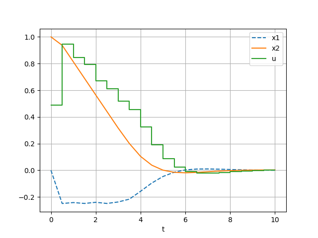
ocp.plot_results(x_opt, u_opt)最终得到
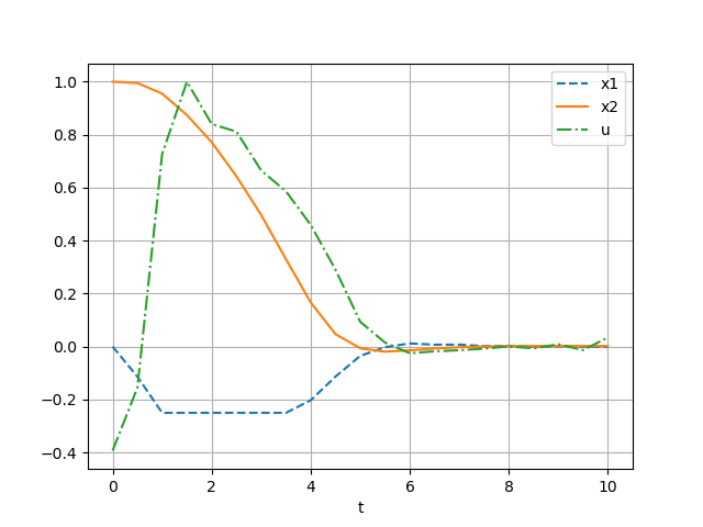
与CasADi给出的标准代码(直接配点法)跑出来的结果进行对比。