探秘Transformer系列之(31)--- Medusa
目录
- [探秘Transformer系列之(31)--- Medusa](#探秘Transformer系列之(31)--- Medusa)
- [0x00 概述](#0x00 概述)
- [0x01 原理](#0x01 原理)
- [1.1 动机](#1.1 动机)
- [1.2 借鉴](#1.2 借鉴)
- [1.3 思路](#1.3 思路)
- [1.3.1 单模型 & 多头](#1.3.1 单模型 & 多头)
- [1.3.2 Tree 验证](#1.3.2 Tree 验证)
- [1.3.3 小结](#1.3.3 小结)
- [0x02 设计核心点](#0x02 设计核心点)
- [2.1 流程](#2.1 流程)
- [2.2 模型结构](#2.2 模型结构)
- [2.3 多头](#2.3 多头)
- [2.3.1 head结构](#2.3.1 head结构)
- [2.3.2 位置](#2.3.2 位置)
- [2.4 缺点](#2.4 缺点)
- [0x03 Tree Verification](#0x03 Tree Verification)
- [3.1 解码路径](#3.1 解码路径)
- [3.2 最佳构造方式](#3.2 最佳构造方式)
- [3.3 实现](#3.3 实现)
- [3.4 Typical Acceptance](#3.4 Typical Acceptance)
- [3.4.1 常见采用方法](#3.4.1 常见采用方法)
- [3.4.2 思路](#3.4.2 思路)
- [3.4.3 Typical Acceptance](#3.4.3 Typical Acceptance)
- [0x04 训练](#0x04 训练)
- [4.1 MEDUSA-1](#4.1 MEDUSA-1)
- [4.2 MEDUSA-2](#4.2 MEDUSA-2)
- [4.3 代码](#4.3 代码)
- [0x05 Decoding](#0x05 Decoding)
- [5.1 示例](#5.1 示例)
- [5.2 计算和空间复杂度](#5.2 计算和空间复杂度)
- [0xFF 参考](#0xFF 参考)
0x00 概述
Medusa 是自投机领域较早的一篇工作,对后续工作启发很大,其主要思想是multi-decoding head + tree attention + typical acceptance(threshold)。Medusa 没有使用独立的草稿模型,而是在原始模型的基础上增加多个解码头(MEDUSA heads),并行预测多个后续 token。
正常的LLM只有一个用于预测t时刻token的head。Medusa 在 LLM 的最后一个 Transformer层之后保留原始的 LM Head,然后额外增加多个(假设是k个) 可训练的Medusa Head(解码头),分别负责预测t+1,t+2,...,和t+k时刻的不同位置的多个 Token。Medusa 让每个头生成多个候选 token,而非像投机解码那样只生成一个候选。然后将所有的候选结果组装成多个候选序列,多个候选序列又构成一棵树。再通过树注意力机制并行验证这些候选序列。
注:全部文章列表在这里,估计最终在35篇左右,后续每发一篇文章,会修改此文章列表。
cnblogs 探秘Transformer系列之文章列表
0x01 原理
1.1 动机
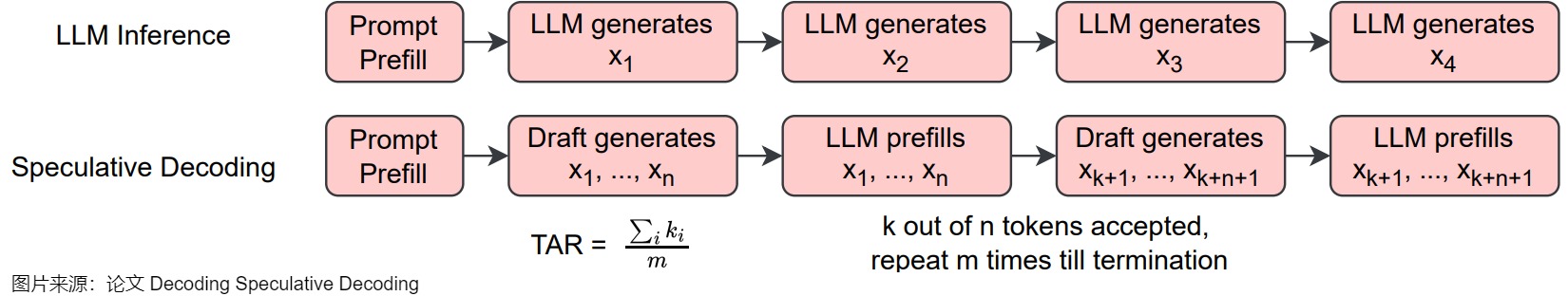
投机采样的核心思路如上图下方所示,首先以低成本的方式(一般来说是用小模型)快速生成多个候选 Token,然后通过一次并行验证阶段快速验证多个 Token,进而减少大模型的 Decoding Step,实现加速的目的。然而,采用一个独立的"推测"模型也有缺点,具体如下:
- 很难找到一个小而强的模型来生成对于原始的模型来说比较简单的token。
- draft模型和大模型很难对齐,存在distribution shift。
- 并不是所有的LLM都能找到现成的小模型。重新训练一个小模型需要较多的额外投入。
- 在一个系统中维护2个不同的模型,即增加了推理过程的计算复杂度,也导致架构上的复杂性,在分布式系统上的部署难度增大。
- 使用投机采样的时候,会带来额外的解码开销,尤其是当使用一个比较高的采样温度值时。
1.2 借鉴
Medua主要借鉴了两个工作:BPD和SpecInfer。
-
大模型自身带有一个LM head,用于把隐藏层输出映射到词表的概率分布,以实现单个token的解码。为了生成多个token,论文"Blockwise Parallel Decoding for Deep Autoregressive Models"在骨干模型上使用多个解码头来加速推理,通过训练辅助模型,使得模型能够预测未来位置的输出,然后利用这些预测结果来跳过部分贪心解码步骤,从而加速解码过程。
-
论文"SpecInfer: Accelerating Generative Large Language Model Serving with Speculative Inference and Token Tree Verification"的思路是:既然小模型可以猜测大模型的输出并且效率非常高,那么一样可以使用多个小模型来猜测多个 Token 序列,这样提供的候选更多,猜对的机会也更大;为了提升这多个 Token 序列的验证效率,作者提出 Token Tree Attention 的机制,首先将多个小模型生成的多个 Token 序列组合成 Token 树,然后将其展开输入模型,即可实现一次 decoding step 完成整个 Token 树的验证。
1.3 思路
基于这两个思路来源,Medusa决定让target LLM自己进行预测,即在target LLM最后一层decoder layer之上引入了多个额外的预测头,使得模型可以在每个解码步并行生成多个token,作为"推测"结果。我们进行具体分析。
1.3.1 单模型 & 多头
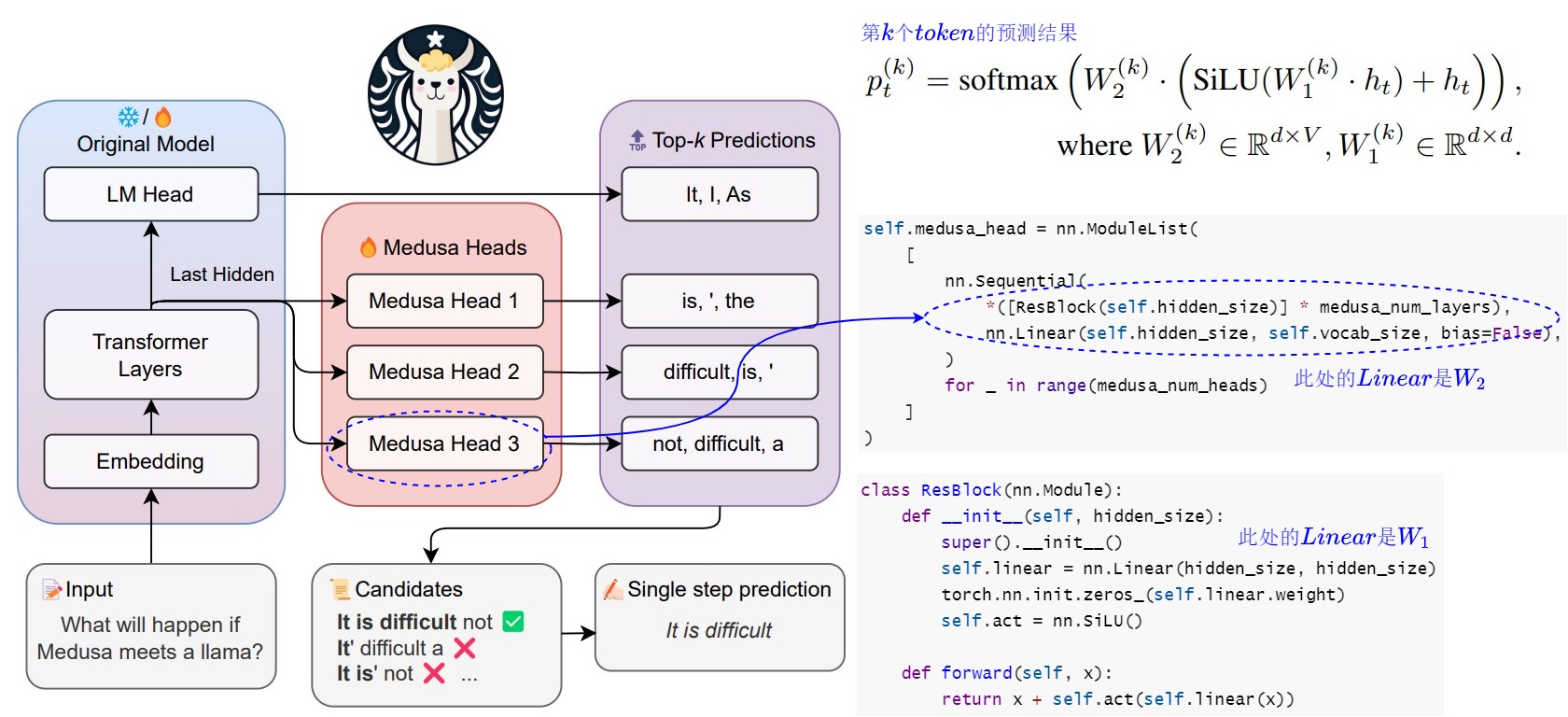
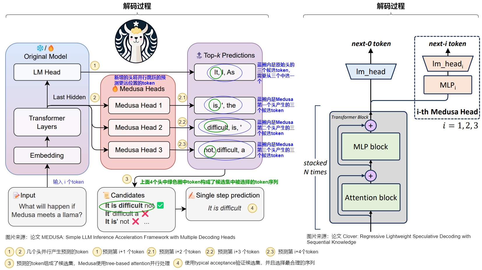
为了抛弃独立的 Draft Model,只保留一个模型,同时保留 Draft-then-Verify 范式,Medusa 在主干模型的最终隐藏层之后添加了若干个 Medusa Heads,每个解码头是一个带残差连接的单层前馈网络。这些Medusa Heads是对BPD中多 Head 的升级,即由原来的一个 Head 生成一个 Token 变成一个 head 生成多个候选 Token。因为这些 Heads 具有预测对应位置 token 的能力,并且可以并行地执行,因此可以实现在一次前向中得到多个 draft tokens。具体如下图所示。
可能有读者会有疑问,后面几个head要跨词预测,其准确率应该很难保证吧?确实是这样的,但是,如果我每个预测时间步都取top3出来,那么最终预测成功的概率就高不少了。而且,Medusa 作者观察到,虽然在预测 next next Token 的时候 top1 的准确率可能只有 60%,但是如果选择 top5,则准确率有可能超过 80%。而且,因为 MEDUSA 解码头与原始模型共享隐藏层状态,所以分布差异较小。

1.3.2 Tree 验证
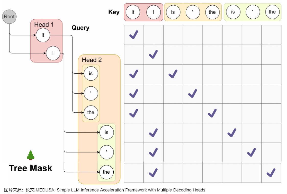
因为贪心解码的正确率不够高,加速效果不够显著,因此Medusa让每个Head解码top-k个候选,不同head的候选集合组成一个树状结构。为了更高效地验证这些 draft tokens,Medusa根据这些 Head 生成 Token 的笛卡尔积来构建出多个 Token 序列。然后使用Tree Attention方法,在注意力计算中,只允许同一延续中的 token 互相看到(attention mask),再加上位置编码的配合,就可以在不增加 batch size 的情况下并行处理多个候选。
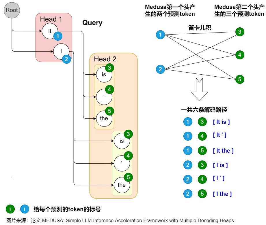
Medusa 中的树和注意力掩码矩阵如下图所示。在每一跳中,我们看到图中Medusa保留了多个可能的token,也就是概率最高的几个token。这样构成了所谓的树结构,直观来说,就是每1跳的每1个token都可能和下1跳的所有token组合成句子,也可以就在这1跳终止。例如,在图中,一共2个head生成了2跳的token,那么这棵树包含了6种可能的句子:Head 1 在下一个位置生成 2 个可能的 Token(It 和 I),Head 2 在下下一个位置生成 3 个可能的 Token(is,' 和 the),这样下一个位置和下下一个位置就有了 2 x 3 = 6 种可能的候选序列,如下图左侧所示。
而其对应的 Attention Mask 矩阵如右侧所示。与原始投机解码略有不同的地方是,树中有多条解码路径,不同解码路径之间不能相互访问。比如,(1) "It is"和 (2) "I is"是两条路径,那么在计算(1).is的概率分布时,只能看到(1).it,而不能看到(2)中的"I"。因此,Medusa新建了在并行计算多条路径概率分布时需要的attention mask,称为"Tree attention"。本质上就是同一条路径内遵从因果mask的规则,不同路径之间不能相互访问。
Medusa作者称,SpecInfer中每个speculator生成称的序列长度不同,所以Mask是动态变化的。而Medusa的Tree Attention Mask在Infrence过程中是静态不变的,这使得对树注意力Mask的预处理进一步提高了效率。

1.3.3 小结
下表给出了BPD,SpecInfer,Medusa之间的差异。
| 领域 | Blockwise Parallel Decoding | SpecInfer | Medusa |
|---|---|---|---|
| 多模型 | 没有真的构造出k-1个辅助模型,只对原始模型略作改造,让其具备预测后k个token的能力 | 采用一批small speculative models(SSMs),并行预测多个候选SSM,可以是原始LLM的蒸馏、量化、剪枝版本 | |
| 多头 | 加入k个project layer,这k个project layer的输出就是k个不同位置token的logits | 在 LLM 的最后一个 Transformer Layer 之后保留原始的 LM Head,然后额外增加多个 Medusa Head,获得多个候选的 Token 序列 | |
| Tree | 将SSMs预测的多个候选merge为一个新的token tree,采用原始LLM做并行验证。SpecInfer中每个speculator生成称的序列长度不同,所以Mask是动态变化的。 | Medusa的Tree Attention Mask在Infrence过程中是静态不变的,这使得对树注意力Mask的预处理进一步提高了效率。 | |
| 训练 | 重新训练原始模型 | 训练小模型 | 并不需要重新训练整个大模型,而是冻结大模型而只训练解码头 |
0x02 设计核心点
2.1 流程
MEDUSA的大致思路和投机解码类似,其中每个解码步骤主要由三个子步骤组成:
- 生成候选者。MEDUSA通过接在原模型的多个Medusa解码头来获取多个位置的候选token
- 处理候选者。MEDUSA把各个位置的候选token进行处理,选出一些候选序列。然后通过tree attention来进行验证。由于 MEDUSA 头位于原始模型之上,因此,此处计算的 logits可以用于下一个解码步骤。
- 接受候选者。通过typical acceptance(典型接受)来选择最终输出的结果。
Medusa更大的优势在于,除了第一次Prefill外,后续可以达到边verify边生成的效果,即 Medusa 的推理流程可以理解:Prefill + Verify + Verify + ...。
2.2 模型结构
下面代码给出了美杜莎的模型结构。Medusa 是在 LLM 的最后一个 Transformer Layer 之后保留原始的 LM Head,然后额外加多个 Medusa Head,也就是多个不同分支输出。这样可以预测出多个候选的 Token 序列。
Medusa head的输入是大模型的隐藏层输出。这是和使用外挂小模型投机解码的另一个重要不同。外挂小模型的输入是查表得到的token embedding,比这里的大模型最后一层隐藏层要弱的多,因此比较依赖小模型的性能。正是因为借助大模型的隐藏层输出,这里的Medusa head的结构都十分简单。
python
class MedusaLlamaModel(KVLlamaForCausalLM):
    """The Medusa Language Model Head.
    This module creates a series of prediction heads (based on the 'medusa' parameter)
    on top of a given base model. Each head is composed of a sequence of residual blocks
    followed by a linear layer.
    """

    def __init__(
        self,
        config,
    ):
        # Load the base model
        super().__init__(config)
        # For compatibility with the old APIs

        medusa_num_heads = config.medusa_num_heads
        medusa_num_layers = config.medusa_num_layers
        base_model_name_or_path = config._name_or_path
        self.hidden_size = config.hidden_size
        self.vocab_size = config.vocab_size
        self.medusa = medusa_num_heads
        self.medusa_num_layers = medusa_num_layers
        self.base_model_name_or_path = base_model_name_or_path
        self.tokenizer = AutoTokenizer.from_pretrained(self.base_model_name_or_path)
        # Create a list of Medusa heads
        self.medusa_head = nn.ModuleList(
            [
                nn.Sequential(
                    *([ResBlock(self.hidden_size)] * medusa_num_layers),
                    nn.Linear(self.hidden_size, self.vocab_size, bias=False),
                )
                for _ in range(medusa_num_heads)
            ]
        )


    def forward(
        self,
        input_ids=None,
        attention_mask=None,
        past_key_values=None,
        output_orig=False,
        position_ids=None,
        medusa_forward=False,
        **kwargs,
    ):
        """Forward pass of the MedusaModel.

        Args:
            input_ids (torch.Tensor, optional): Input token IDs.
            attention_mask (torch.Tensor, optional): Attention mask.
            labels (torch.Tensor, optional): Ground truth labels for loss computation.
            past_key_values (tuple, optional): Tuple containing past key and value states for attention.
            output_orig (bool, optional): Whether to also output predictions from the original LM head.
            position_ids (torch.Tensor, optional): Position IDs.

        Returns:
            torch.Tensor: A tensor containing predictions from all Medusa heads.
            (Optional) Original predictions from the base model's LM head.
        """
        if not medusa_forward:
            return super().forward(
                input_ids=input_ids,
                attention_mask=attention_mask,
                past_key_values=past_key_values,
                position_ids=position_ids,
                **kwargs,
            )
        with torch.inference_mode():
            # Pass input through the base model
            outputs = self.base_model.model(
                input_ids=input_ids,
                attention_mask=attention_mask,
                past_key_values=past_key_values,
                position_ids=position_ids,
                **kwargs,
            )
            if output_orig:
                # 原始模型输出
                orig = self.base_model.lm_head(outputs[0])
        # Clone the output hidden states
        hidden_states = outputs[0].clone()
        medusa_logits = []
        # TODO: Consider parallelizing this loop for efficiency?
        for i in range(self.medusa):
            # 美杜莎头输出
            medusa_logits.append(self.medusa_head[i](hidden_states))
        if output_orig:
            return torch.stack(medusa_logits, dim=0), outputs, orig
        return torch.stack(medusa_logits, dim=0)
2.3 多头
2.3.1 head结构
Medusa 额外新增 medusa_num_heads 个 Medusa Head,每个 Medusa Head 是一个加上了残差连接的单层前馈网络,其中的 Linear 和模型的默认 lm_head 维度一样,这样可以预测后续的 Token。
python
self.medusa_head = nn.ModuleList(
    [
        nn.Sequential(
            *([ResBlock(self.hidden_size)] * medusa_num_layers),
            nn.Linear(self.hidden_size, self.vocab_size, bias=False),
        )
        for _ in range(medusa_num_heads)
    ]
)
下面代码为打印出来的实际内容。
python
ModuleList(
(0-3): 4 x Sequential(
(0): ResBlock(
(linear): Linear(in_features=4096, out_features=4096, bias=True)
(act): SiLU()
)
(1): Linear(in_features=4096, out_features=32000, bias=False)
)
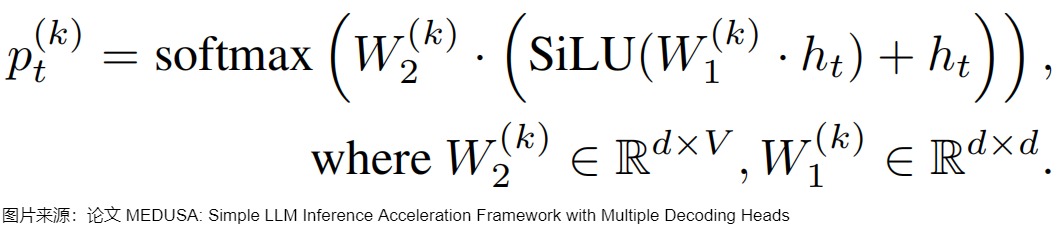
)把第k个解码头在词表上的输出分布记作 \(p_t^{(t)}\),其计算方式如下。d是hidden state的输出维度,V是词表大小,原始模型的预测表示为 \(p_t^{(0)}\) 。
下面是把代码和模型结构结合起来的示意图。
2.3.2 位置
Medusa每个头预测的偏移量是不同的,第k个头用来预测位置t+k+1的输出token(k的取值是1~K)。原模型的解码头依然预测位置t+1的输出,相当于k=0。具体而言,把原始模型在位置t的最后隐藏状态 \(ℎ_t\)接入到K个解码头上,对于输入token序列 \(t_0,t_1,..,t_i\),原始的head根据输入预测 t_{i+1},Medusa新增的第一个head根据输入预测 \(t_{i+2}\)的token,也就是跳过token \(t_{i+1}\) 预测下一个未来的token。并且每个头可以指定topk个结果。这些头的预测结果构成了多个候选词汇序列,然后利用树形注意力机制同时处理这些候选序列。在每个解码步,选择最长被接受的候选序列作为最终的预测结果。这样,每步可以预测多个词汇,从而减少了总的解码步数,提高了推理速度。
如下图所示,Medusa在原始模型基础上,增加了3个额外的Head,可以并行预测出后4个token的候选。
2.4 缺点
Medusa的缺点如下:
- Medusa 新增的 lm_head 和最后一个 Transformer Block 中间只有一个 MLP,表达能力可能有限。
- Medusa 增加了模型参数量,会增加显存占用;
- Medusa 每个 head 都是独立执行的,也就是 "next next token" 预测并不会依赖上一个 "next token" 的结果,导致生成效果不佳,接受率比较低,在大 batch size 时甚至可能负优化。
- 缺乏序列依赖也可能导致低效的树剪枝算法。
- 草稿质量仍然不高,加速效果有限,并且在非贪婪解码 (non-greedy decoding) 下不能保证输出分布与目标LLM一致。
因此,后续有研究工作对此进行了改进。比如Clover重点是提供序列依赖和加入比单个 MLP 具有更强的表征能力的模块。Hydra 增加了 draft head 预测之间的关联性。Hydra++使用 base model 的输出预测概率作为知识蒸馏的教师模型输出来训练 draft head。并且类似EAGLE,Hydra++增加一个独立的 decoder layer,每个 Hydra head 除了上一个 token 本身,还添加了上一个 token 在这个 decoder layer 的 representation 作为输入。
0x03 Tree Verification
每个Medusa Head 会生成 top-k 个预测标记,然后通过计算这些预测的笛卡尔积来形成候选序列。我们可以对于每个候选序列都走一遍模型来验证,但是这样做太耗时。因此,Medusa 作者设计了一种tree attention的机制,在候选树内进行掩码操作,掩码限制某个token对前面token的注意力。同时,也要为相应地为position embedding设置正确的位置索引。因为有 tree attention 的存在,所以 Medusa 可以并行地构建、维护和验证多个候选序列。
3.1 解码路径
在Medusa中,基础版本解码采用greedy方式取Top-1 Token。Medusa增加额外的解码头之后,使用 Top-K Sampling,每一个 Head 都会输出 k 个 tokens。不同Medusa头之间预测结果不一致。\(p(t_{t+1}|t_0,...,t_i)\)和\(p(t_{t+2}|t_0,...,t_i)\)形式上是条件独立的,但是实际上\(p_{t+2}\)依赖\(p_{t+1}\),不能直接取\(p(t_{t+1}|t_0,...,t_i)\)和\(p(t_{t+2}|t_0,...,t_i)\)最大的token作为verify阶段的输入,这样组成的句子可能会在逻辑上不一致。因此,Medusa还引入采样topk组合作为候选序列的方式去缓解这个问题。最终把LM_head 的输出作为根节点构建出树状结构,树的深度自顶向下遍历称为解码路径(论文中叫做candidates path)。每个候选序列可以表示所构建的tree上的一条路径上所有的node(而不只是leaf node,因为tree attention验证的时候会把路径上所有token都进行验证)。
在构建树形结构时,最简单的方法是通过笛卡尔积来获取多个解码头组成的所有可能的候选序列。下图例子使用了Cartesian product对两个解码头的结果进行处理,获得所有候选序列。具体来说就是将每个头的top-k个词作为节点,每个头作为树的一层。图上一共存在6条解码路径,相当于 Head 1 在下一个位置生成 2 个可能的 Token(It 和 I),Head 2 在下下一个位置生成 3 个可能的 Token(is,' 和 the),这样下一个位置和下下一个位置就有了 2 x 3 = 6 种可能的候选序列。为了区分不同的 prefix,Medusa 设置了一些冗余,例如 Head 2 的三个预测 token 均出现了两次,这是为了分别对应 It 和 I 这两个不同的 prefix。每个 token 在 tree mask 的作用下只可以看见自己的 prefix。
3.2 最佳构造方式
上图采用top-3,两个头一共有6条候选路径。如果解码头数量数量比较多,每个头给出的候选token也比较多。解码路径会随着Top-k 和头数增多急剧增加,会产生大量的候选路径,具有庞大的搜索空间。虽然增加候选序列的数量,最终接受token的命中率就会提升,但是验证更多候选序列也会带来额外的计算消耗。那么新的问题是:
- 如何能减少候选解码路径?
- 如何能在候选解码路径中,得到最优解码路径?
直观上来说,那些由不同头部的topk预测组成的候选结果可能具有不同的准确率。应该优先选择那些更准确的预测,从而构建一个更有效的树,而不需要使用所有可能的排列组合。Medusa 通过在校准数据集上统计每个解码头的 top-k 预测的准确率,然后贪婪地选择那些能够最大化期望接受长度的节点,将它们加入到树中。这样可以在相同的节点总数下,获得更高的加速比。
具体来说,我们可以使用一个calibration dataset(比如Alpaca-eval dataset)来获取不同解码头给出的各个token的准确率:把第 k 个解码头给出的第 i 个token的准确率记为 \(a_k^{(i)}\)。假设各个token的准确率之间是独立的,那么一个由\[i_1,i_2,\\cdots,i_k\] 构成的候选序列的准确率可以写作 \(\prod_{j=1}^ka_j^{(i_j)}\)。我们用 I 表示候选序列的集合,那么集合里的候选序列的expectation of acceptance length就表示为:
\\\sum_{\[i_1,i_2,\\cdots,i_k\in I}\prod_{j=1}^ka_j^{(i_j)} \]
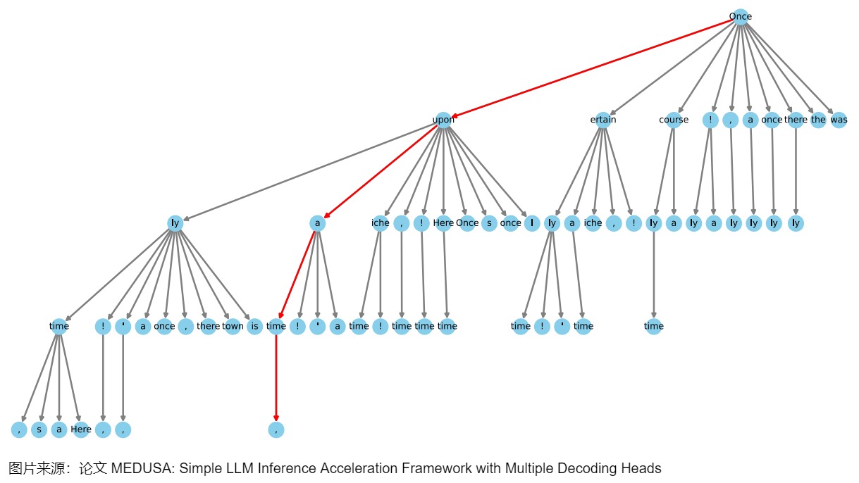
在构建tree的时候,Medusa 用贪心算法优先加入当前有最大准确率的候选序列,直到tree的节点数量达到接受长度的期望值上限,这样能最大化expectation of acceptance length,也就能最大化acceleration rate。这是一种手工设计的稀疏树结构,越靠前的节点,有更多的子节点路径。MEDUSA-2 Vicuna-7B模型的一个稀疏树示例如下图所示。这个树结构延伸了四个层次,表明有四个MEDUSA头参与了计算。该树最初通过笛卡尔积方法生成,随后根据每个MEDUSA头在Alpaca-eval数据集上测量的前 k 个预测的统计期望值进行修剪。树向左倾斜在视觉上代表了算法倾向于使用更高准确率的token,每个节点表示MEDUSA头部的top-k预测中的一个token,边显示了它们之间的连接,红线突出显示了正确预测未来token的路径。这样就将1000个路径的树优化到只有42条路径,而且,这里的路径可以提前结束,不要求一定要遍历到最后一层。
3.3 实现
3.3.1 关键变量
我们首先看看注意力树所涉及的关键变量。
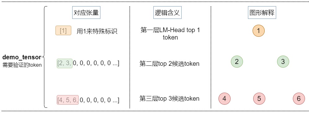
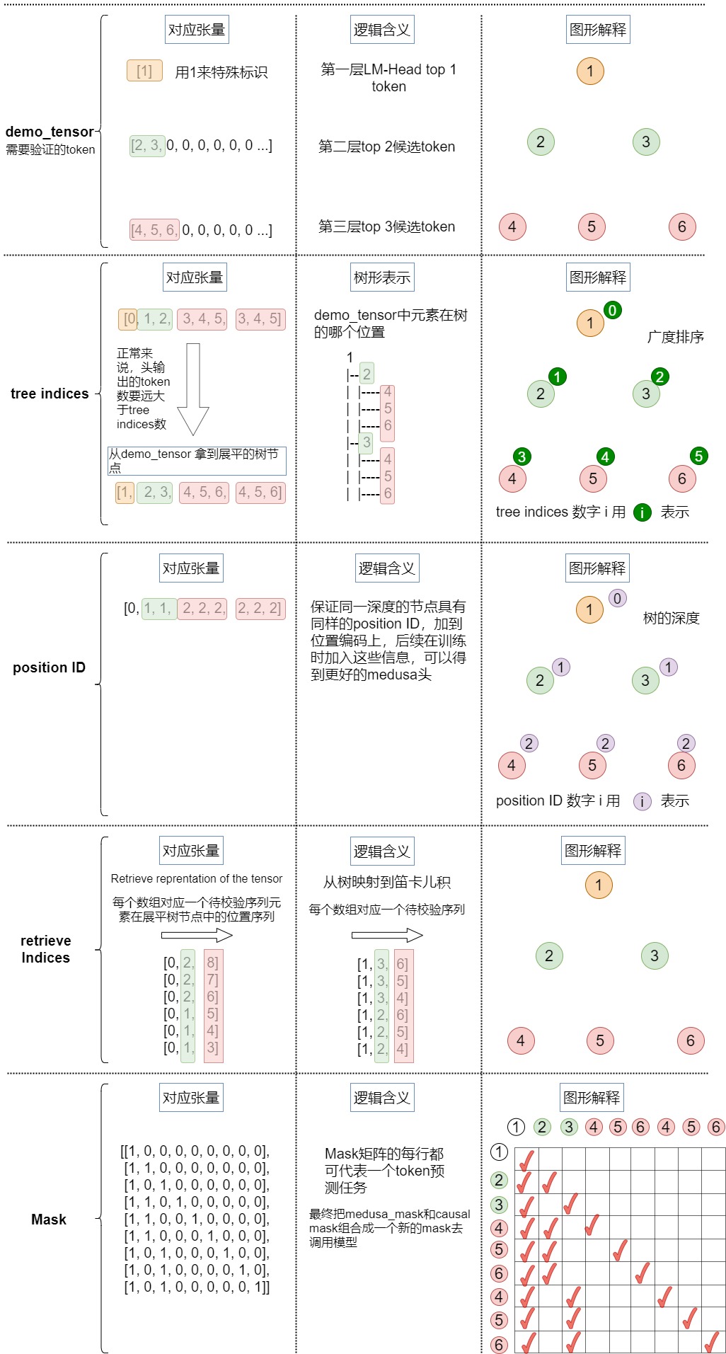
demo_tensor
demo_tensor是输入张量,例子如下:
python
[2, 3, 0, 0, 0, 0, 0, 0 ...] # 1st depth we choose top 2
[4, 5, 6, 0, 0, 0, 0, 0 ...] # 2nd depth we choose top 3
对应下图。
medusa_choices
medusa_choices是一个嵌套列表,表示medusa树结构,决定解码路径。外部列表对应于树中的节点,每个内部列表给出该节点在树中的祖先及其位置。根据Medusa choies 我们可以构建稀疏树的所有数据成员,源码中的例子如下。
python
vicuna_7b_stage2 = [(0,), (0, 0), (1,), (0, 1), (0, 0, 0), (1, 0), (2,), (0, 2), (0, 0, 1), (0, 3), (3,), (0, 1, 0), (2, 0), (4,), (0, 0, 2), (0, 4), (1, 1), (1, 0, 0), (0, 0, 0, 0), (5,), (0, 0, 3), (0, 5), (0, 2, 0), (3, 0), (0, 1, 1), (0, 6), (6,), (0, 7), (0, 0, 4), (4, 0), (1, 2), (0, 8), (7,), (0, 3, 0), (0, 0, 0, 1), (0, 0, 5), (2, 1), (0, 0, 6), (1, 0, 1), (0, 0, 1, 0), (2, 0, 0), (5, 0), (0, 9), (0, 1, 2), (8,), (0, 4, 0), (0, 2, 1), (1, 3), (0, 0, 7), (0, 0, 0, 2), (0, 0, 8), (1, 1, 0), (0, 1, 0, 0), (6, 0), (9,), (0, 1, 3), (0, 0, 0, 3), (1, 0, 2), (0, 5, 0), (3, 1), (0, 0, 2, 0), (7, 0), (1, 4)]
vicuna_7b_stage1_ablation = [(0,), (0, 0), (1,), (0, 0, 0), (0, 1), (1, 0), (2,), (0, 2), (0, 0, 1), (3,), (0, 3), (0, 1, 0), (2, 0), (0, 0, 2), (0, 4), (4,), (0, 0, 0, 0), (1, 0, 0), (1, 1), (0, 0, 3), (0, 2, 0), (0, 5), (5,), (3, 0), (0, 1, 1), (0, 6), (6,), (0, 0, 4), (1, 2), (0, 0, 0, 1), (4, 0), (0, 0, 5), (0, 7), (0, 8), (0, 3, 0), (0, 0, 1, 0), (1, 0, 1), (7,), (2, 0, 0), (0, 0, 6), (2, 1), (0, 1, 2), (5, 0), (0, 2, 1), (0, 9), (0, 0, 0, 2), (0, 4, 0), (8,), (1, 3), (0, 0, 7), (0, 1, 0, 0), (1, 1, 0), (6, 0), (9,), (0, 0, 8), (0, 0, 9), (0, 5, 0), (0, 0, 2, 0), (1, 0, 2), (0, 1, 3), (0, 0, 0, 3), (3, 0, 0), (3, 1)]
vicuna_7b_stage1 = [(0,), (0, 0), (1,), (2,), (0, 1), (1, 0), (3,), (0, 2), (4,), (0, 0, 0), (0, 3), (5,), (2, 0), (0, 4), (6,), (0, 5), (1, 1), (0, 0, 1), (7,), (3, 0), (0, 6), (8,), (9,), (0, 1, 0), (0, 7), (0, 8), (4, 0), (0, 0, 2), (1, 2), (0, 9), (2, 1), (5, 0), (1, 0, 0), (0, 0, 3), (1, 3), (0, 2, 0), (0, 1, 1), (0, 0, 4), (6, 0), (1, 4), (0, 0, 5), (2, 2), (0, 3, 0), (3, 1), (0, 0, 6), (7, 0), (1, 5), (1, 0, 1), (2, 0, 0), (0, 0, 7), (8, 0), (0, 0, 0, 0), (4, 1), (0, 1, 2), (0, 4, 0), (9, 0), (0, 2, 1), (2, 3), (1, 6), (0, 0, 8), (0, 5, 0), (3, 2), (5, 1)]我们此处例子为:[[0], [0, 0], [0, 1], [0, 2], [1], [1, 0], [1, 1], [1, 2]],这里[1]为根节点,则可视化如下。
python
[1]
[2, 3]
[4, 5, 6]
medusa_buffers
medusa_buffers数据结构信息如下。
python
medusa_buffers = generate_medusa_buffers(medusa_choices, device='cpu')

medusa_buffers = {
    "medusa_attn_mask": medusa_attn_mask.unsqueeze(0).unsqueeze(0),
    "tree_indices": medusa_tree_indices,
    "medusa_position_ids": medusa_position_ids,
    "retrieve_indices": retrieve_indices,
    }
其中成员变量作用如下:
- medusa_attn_mask:就是树注意力用到的掩码。
- tree_indices:demo_tensor中元素在树的哪个位置,在 generate_candidates()函数中会用到。
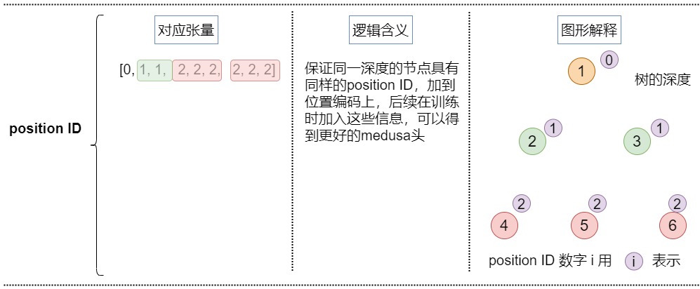
- medusa_position_ids:保证同一深度的节点具有同样的position ID,加到位置编码上,后续在训练时加入这些信息,可以得到更好的medusa头。在tree_decoding()函数中用到。
- retrieve_indices:从树映射到笛卡尔积,代表每个笛卡尔积在logits中的位置。依据这些信息,可以从logits里面提取每个笛卡尔积对应的logits。在tree_decoding()函数和generate_candidates()函数中用到。
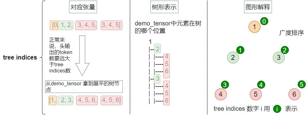
tree_indices
tree_indices代表demo_tensor中元素在树的哪个位置。对于给定的输入张量,对应的tree_indices如下。
python
[0, 1, 2, 3, 4, 5, 3, 4, 5]长成的树如下。
python
1
|-- 2
|  |-- 4
|  |-- 5
|  |-- 6
|-- 3
|  |-- 4
|  |-- 5
|  |-- 6
从demo_tensor 拿到展平的树节点如下。
python
[1, 2, 3, 4, 5, 6, 4, 5, 6]参见下图。
medusa_position_ids
medusa_position_ids:保证同一深度的节点具有同样的position ID。加入这些信息之后,每个token对应的位置编码是:序列中的位置 + 树中的深度。这样在后续训练medusa头时就知道深度信息,可以训练出更好的medusa头。在tree_decoding()函数中用到此变量。
输入张量对应的位置id如下。
python
[0, 1, 1, 2, 2, 2, 2, 2, 2] # Medusa position IDs
 |  |  |  |  |  |  |  |  |
[1, 2, 3, 4, 5, 6, 4, 5, 6] # Flatten tree representation of the tensor
可视化如下。
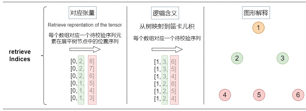
retrieve_indices
retrieve_indices是从树映射到笛卡尔积,代表每个笛卡尔积在logits中的位置。依据这些信息,可以从logits里面提取每个笛卡尔积对应的logits。
本例的retrieve_indices如下。
python
[0, 2, 8]
[0, 2, 7]
[0, 2, 6]
[0, 1, 5]
[0, 1, 4]
[0, 1, 3]
把树映射到笛卡尔积之后如下。
python
[1, 3, 6]
[1, 3, 5]
[1, 3, 4]
[1, 2, 6]
[1, 2, 5]
[1, 2, 4]
具体可视化如下。
medusa_attn_mask
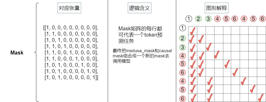
因为最终组成的树是将每个头的top-k个词作为节点,每个头作为树的一层,每条直到叶子节点的路径构成一组待验证的预测。在这棵树内,Attention Mask需要新的设计,该Mask只限制一个token对前面token的注意力。同时,要为相应地为position embedding设置正确的位置索引。掩码矩阵的细节如下:
Mask矩阵的每行都可以代表一个token预测任务- 在
Tree Mask矩阵中,需要对位置编码进行错位编码
论文中例子如下。
对于本例的掩码如下。
3.3.2 示例代码
示例代码如下
python
demo_tensor = torch.zeros(2,10).long()
demo_tensor[0,0] = 2
demo_tensor[0,1] = 3
demo_tensor[1,0] = 4
demo_tensor[1,1] = 5
demo_tensor[1,2] = 6
print('Demo tensor: \n', demo_tensor)
demo_tensor = demo_tensor.flatten()
demo_tensor = torch.cat([torch.ones(1).long(), demo_tensor])
print('='*50)
medusa_choices = [[0], [0, 0], [0, 1], [0, 2], [1], [1, 0], [1, 1], [1, 2]]
medusa_buffers = generate_medusa_buffers(medusa_choices, device='cpu')
tree_indices = medusa_buffers['tree_indices']
medusa_position_ids = medusa_buffers['medusa_position_ids']
retrieve_indices = medusa_buffers['retrieve_indices']
print('Tree indices: \n', tree_indices.tolist())
print('Tree reprentation of the tensor: \n', demo_tensor[tree_indices].tolist())
print('='*50)
print('Medusa position ids: \n', medusa_position_ids.tolist())
print('='*50)
print('Retrieve indices: \n', retrieve_indices.tolist())
demo_tensor_tree = demo_tensor[tree_indices]
demo_tensor_tree_ext = torch.cat([demo_tensor_tree, torch.ones(1).long().mul(-1)])
print('Retrieve reprentation of the tensor: \n', demo_tensor_tree_ext[retrieve_indices].tolist())
print('='*50)
demo_tensor_tree_ext[retrieve_indices].tolist()
print('='*50)
print(medusa_buffers['medusa_attn_mask'][0,0,:,:].int())
print('='*50)
print(medusa_buffers['medusa_attn_mask'][0,0,:,:].int())
打印结果:
python
Demo tensor:
 tensor([[2, 3, 0, 0, 0, 0, 0, 0, 0, 0],
        [4, 5, 6, 0, 0, 0, 0, 0, 0, 0]])
==================================================
Tree indices:
 [0, 1, 2, 11, 12, 13, 11, 12, 13]
Tree reprentation of the tensor:
 [1, 2, 3, 4, 5, 6, 4, 5, 6]
==================================================
Medusa position ids:
 [0, 1, 1, 2, 2, 2, 2, 2, 2]
==================================================
Retrieve indices:
 [[0, 2, 8], [0, 2, 7], [0, 2, 6], [0, 1, 5], [0, 1, 4], [0, 1, 3]]
Retrieve reprentation of the tensor:
 [[1, 3, 6], [1, 3, 5], [1, 3, 4], [1, 2, 6], [1, 2, 5], [1, 2, 4]]
==================================================
tensor([[1, 0, 0, 0, 0, 0, 0, 0, 0],
        [1, 1, 0, 0, 0, 0, 0, 0, 0],
        [1, 0, 1, 0, 0, 0, 0, 0, 0],
        [1, 1, 0, 1, 0, 0, 0, 0, 0],
        [1, 1, 0, 0, 1, 0, 0, 0, 0],
        [1, 1, 0, 0, 0, 1, 0, 0, 0],
        [1, 0, 1, 0, 0, 0, 1, 0, 0],
        [1, 0, 1, 0, 0, 0, 0, 1, 0],
        [1, 0, 1, 0, 0, 0, 0, 0, 1]], dtype=torch.int32)
3.3.3 总体可视化
具体可视化参见下图。
3.3.4 使用
调用
整体调用代码如下。基本逻辑是:
- 根据设定的medusa choices得到稀疏的树结构表达,具体涉及generate_medusa_buffers()函数。
- 初始化key和value。
- 构建树注意力掩码,根据输入的 Prompt 进行预测,输出 logits 和 medusa_logits。具体涉及initialize_medusa()函数。logits对应 lm_head 的输出,medusa_logits对应medusa_head 的输出。
- 从树中提取用美杜莎头得到的topk预测。这些预测构成了候选路径。具体涉及generate_candidates()函数。
- 用树注意力验证候选路径,得到最佳路径。具体涉及tree_decoding()函数和evaluate_posterior()函数。tree_decoding()函数执行基于树注意力(tree-attention-based)的推理。evaluate_posterior()函数执行对树的验证。
- 根据候选 Token 序列选出对应的 logits,medusa_logits,并更新输入,key、value cache 等。具体涉及update_inference_inputs()函数。
python
def medusa_forward(input_ids, model, tokenizer, medusa_choices, temperature, posterior_threshold, posterior_alpha, top_p=0.8, sampling = 'typical', fast = True, max_steps = 512):

    # Avoid modifying the input_ids in-place
    input_ids = input_ids.clone()

    # Cache medusa buffers (the fixed patterns for tree attention)
    if hasattr(model, "medusa_choices") and model.medusa_choices == medusa_choices:
        # Load the cached medusa buffer
        medusa_buffers = model.medusa_buffers
    else:
        # Initialize the medusa buffer
        # 1. 根据设定的medusa choices得到稀疏的树结构表达
        medusa_buffers = generate_medusa_buffers(
            medusa_choices, device=model.base_model.device
        )
    model.medusa_buffers = medusa_buffers
    model.medusa_choices = medusa_choices

    # Initialize the past key and value states
    if hasattr(model, "past_key_values"):
        past_key_values = model.past_key_values
        past_key_values_data = model.past_key_values_data
        current_length_data = model.current_length_data
        # Reset the past key and value states
        current_length_data.zero_()
    else:
        (
            past_key_values,
            past_key_values_data,
            current_length_data,
        ) = initialize_past_key_values(model.base_model)
        model.past_key_values = past_key_values
        model.past_key_values_data = past_key_values_data
        model.current_length_data = current_length_data

    input_len = input_ids.shape[1]
    reset_medusa_mode(model)

    # Initialize tree attention mask and process prefill tokens
    medusa_logits, logits = initialize_medusa(
            input_ids, model, medusa_buffers["medusa_attn_mask"], past_key_values
    )
    new_token = 0

    for idx in range(max_steps):
        # Generate candidates with topk predictions from Medusa heads
        # 用美杜莎头得到的topk预测来生成候选路径。candidates是多个候选 Token 序列。tree_candidates是Token 树
        candidates, tree_candidates = generate_candidates(
                medusa_logits,
                logits,
                medusa_buffers["tree_indices"],
                medusa_buffers["retrieve_indices"],
                temperature, posterior_threshold, posterior_alpha, top_p, sampling, fast
            )
        # Use tree attention to verify the candidates and get predictions
        # 用树注意力验证候选路径。使用 Tree Attention 机制对 tree_candidates 进行验证推理,获得新的 logits 和 medusa_logits 输出。
        medusa_logits, logits, outputs = tree_decoding(
                model,
                tree_candidates,
                past_key_values,
                medusa_buffers["medusa_position_ids"],
                input_ids,
                medusa_buffers["retrieve_indices"],
            )
        # 评估每条路径合理性,得到最佳路径。如果所有序列都没有通过,则只使用第一个 Token,对应 accept_length 为 0,如果某个序列通过,则使用该序列中的已接受的 Token
        best_candidate, accept_length = evaluate_posterior(
                logits, candidates, temperature, posterior_threshold, posterior_alpha , top_p, sampling, fast
            )
        # 根据候选 Token 序列选出对应的 logits,medusa_logits,并更新输入,key、value cache 等
        input_ids, logits, medusa_logits, new_token = update_inference_inputs(
                input_ids,
                candidates,
                best_candidate,
                accept_length,
                medusa_buffers["retrieve_indices"],
                outputs,
                logits,
                medusa_logits,
                new_token,
                past_key_values_data,
                current_length_data,
            )
        if tokenizer.eos_token_id in input_ids[0, input_len:].tolist():
            break
        if new_token > 1024:
            break
    return input_ids, new_token, idx
初始化
initialize_medusa()函数会进行初始化操作,得到logits和mask。
python
def initialize_medusa(input_ids, model, medusa_attn_mask, past_key_values):
    """
    Initializes the Medusa structure for a given model.

    This function performs the following operations:
    1. Forward pass through the model to obtain the Medusa logits, original model outputs, and logits.
    2. Sets the Medusa attention mask within the base model.

    Args:
    - input_ids (torch.Tensor): The input tensor containing token ids.
    - model (MedusaLMHead): The model containing the Medusa layers and base model.
    - medusa_attn_mask (torch.Tensor): The attention mask designed specifically for the Medusa structure.
    - past_key_values (list of torch.Tensor): Contains past hidden states and past attention values.

    Returns:
    - medusa_logits (torch.Tensor): Logits from the Medusa heads.
    - logits (torch.Tensor): Original logits from the base model.
    """
    medusa_logits, outputs, logits = model(
        input_ids, past_key_values=past_key_values, output_orig=True, medusa_forward=True
    )
    model.base_model.model.medusa_mask = medusa_attn_mask
    return medusa_logits, logits
在具体模型中,会把medusa_mask和causal mask组合在一起,形成一个新的mask。最终在前向传播时候,传递的就是这个最终组合mask。
python
class LlamaModel(LlamaPreTrainedModel):
    # Copied from transformers.models.bart.modeling_bart.BartDecoder._prepare_decoder_attention_mask
    def _prepare_decoder_attention_mask(
        self, attention_mask, input_shape, inputs_embeds, past_key_values_length
    ):
        # create causal mask
        # [bsz, seq_len] -> [bsz, 1, tgt_seq_len, src_seq_len]
        combined_attention_mask = None
        if input_shape[-1] > 1:
            combined_attention_mask = _make_causal_mask(
                input_shape,
                # inputs_embeds.dtype,
                torch.float32,  # [MODIFIED] force to cast to float32
                device=inputs_embeds.device,
                past_key_values_length=past_key_values_length,
            )

        if attention_mask is not None:
            # [bsz, seq_len] -> [bsz, 1, tgt_seq_len, src_seq_len]
            expanded_attn_mask = _expand_mask(
                attention_mask, inputs_embeds.dtype, tgt_len=input_shape[-1]
            ).to(inputs_embeds.device)
            combined_attention_mask = (
                expanded_attn_mask
                if combined_attention_mask is None
                else expanded_attn_mask + combined_attention_mask
            )

        # [MODIFIED] add medusa mask
        if hasattr(self, "medusa_mask") and self.medusa_mask is not None:
            medusa_mask = self.medusa_mask
            medusa_len = medusa_mask.size(-1)
            combined_attention_mask[:, :, -medusa_len:, -medusa_len:][
                medusa_mask == 0
            ] = combined_attention_mask.min()
            if hasattr(self, "medusa_mode"):
                # debug mode
                if self.medusa_mode == "debug":
                    torch.save(combined_attention_mask, "medusa_mask.pt")

        return combined_attention_mask

    @add_start_docstrings_to_model_forward(LLAMA_INPUTS_DOCSTRING)
    def forward(
        self,
        input_ids: torch.LongTensor = None,
        attention_mask: Optional[torch.Tensor] = None,
        position_ids: Optional[torch.LongTensor] = None,
        past_key_values=None,  # [MODIFIED] past_key_value is KVCache class
        inputs_embeds: Optional[torch.FloatTensor] = None,
        use_cache: Optional[bool] = None,
        output_attentions: Optional[bool] = None,
        output_hidden_states: Optional[bool] = None,
        return_dict: Optional[bool] = None,
    ) -> Union[Tuple, BaseModelOutputWithPast]:

        # ......

        # embed positions
        if attention_mask is None:
            attention_mask = torch.ones(
                (batch_size, seq_length_with_past),
                dtype=torch.bool,
                device=inputs_embeds.device,
            )
        attention_mask = self._prepare_decoder_attention_mask(
            attention_mask,
            (batch_size, seq_length),
            inputs_embeds,
            past_key_values_length,
        )

        # ......

        # decoder layers
        for idx, decoder_layer in enumerate(self.layers):
            if self.gradient_checkpointing and self.training:
				# ......
            else:
                layer_outputs = decoder_layer(
                    hidden_states,
                    attention_mask=attention_mask,
                    position_ids=position_ids,
                    past_key_value=past_key_value,
                    output_attentions=output_attentions,
                    use_cache=use_cache,
                )

            hidden_states = layer_outputs[0]

        hidden_states = self.norm(hidden_states)

        # ......
生成候选路径
generate_candidates()函数的细节如下,主要是预测每个头的topk的token,并且用笛卡尔积组装成可以解析成tree的候选序列。
python
def generate_candidates(medusa_logits, logits, tree_indices, retrieve_indices, temperature = 0, posterior_threshold=0.3, posterior_alpha = 0.09, top_p=0.8, sampling = 'typical', fast = False):
    """
    Generate candidates based on provided logits and indices.

    Parameters:
    - medusa_logits (torch.Tensor): Logits from a specialized Medusa structure, aiding in candidate selection.
    - logits (torch.Tensor): Standard logits from a language model.
    - tree_indices (list or torch.Tensor): Indices representing a tree structure, used for mapping candidates.
    - retrieve_indices (list or torch.Tensor): Indices for extracting specific candidate tokens.
    - temperature (float, optional): Controls the diversity of the sampling process. Defaults to 0.
    - posterior_threshold (float, optional): Threshold for typical sampling. Defaults to 0.3.
    - posterior_alpha (float, optional): Scaling factor for the entropy-based threshold in typical sampling. Defaults to 0.09.
    - top_p (float, optional): Cumulative probability threshold for nucleus sampling. Defaults to 0.8.
    - sampling (str, optional): Defines the sampling strategy ('typical' or 'nucleus'). Defaults to 'typical'.
    - fast (bool, optional): If True, enables faster, deterministic decoding for typical sampling. Defaults to False.

    Returns:
    - tuple (torch.Tensor, torch.Tensor): A tuple containing two sets of candidates:
        1. Cartesian candidates derived from the combined original and Medusa logits.
        2. Tree candidates mapped from the Cartesian candidates using tree indices.
    """
    # Greedy decoding: Select the most probable candidate from the original logits.
    if temperature == 0 or fast:
        candidates_logit = torch.argmax(logits[:, -1]).unsqueeze(0)
    else:
        if sampling == 'typical':
            candidates_logit = get_typical_one_token(logits[:, -1], temperature, posterior_threshold, posterior_alpha).squeeze(0)
        elif sampling == 'nucleus':
            candidates_logit = get_nucleus_one_token(logits[:, -1], temperature, top_p).squeeze(0)
        else:
            raise NotImplementedError
    # Extract the TOPK candidates from the medusa logits.
    candidates_medusa_logits = torch.topk(medusa_logits[:, 0, -1], TOPK, dim = -1).indices

    # Combine the selected candidate from the original logits with the topk medusa logits.
    # 把lm head和medusa heads的logits拼接在一起
    candidates = torch.cat([candidates_logit, candidates_medusa_logits.view(-1)], dim=-1)

    # Map the combined candidates to the tree indices to get tree candidates.
    # 从candidates中拿到树对应的节点
    tree_candidates = candidates[tree_indices]

    # Extend the tree candidates by appending a zero.
    tree_candidates_ext = torch.cat([tree_candidates, torch.zeros((1), dtype=torch.long, device=tree_candidates.device)], dim=0)

    # 从树节点中拿到笛卡尔积
    # Retrieve the cartesian candidates using the retrieve indices.
    cart_candidates = tree_candidates_ext[retrieve_indices]

    # Unsqueeze the tree candidates for dimension consistency.
    tree_candidates = tree_candidates.unsqueeze(0)
    return cart_candidates, tree_candidates
验证候选路径
tree_decoding()函数细节如下。对上面的得到的拉平的序列,用基础的LLM模型预测每一条路径的概率,最后根据retrieve_indices还原到原始的笛卡尔积的路径,可以得到路径上每个位置的概率。
python
def tree_decoding(
    model,
    tree_candidates,
    past_key_values,
    medusa_position_ids,
    input_ids,
    retrieve_indices,
):
    """
    Decode the tree candidates using the provided model and reorganize the logits.

    Parameters:
    - model (nn.Module): Model to be used for decoding the tree candidates.
    - tree_candidates (torch.Tensor): Input candidates based on a tree structure.
    - past_key_values (torch.Tensor): Past states, such as key and value pairs, used in attention layers.
    - medusa_position_ids (torch.Tensor): Positional IDs associated with the Medusa structure.
    - input_ids (torch.Tensor): Input sequence IDs.
    - retrieve_indices (list or torch.Tensor): Indices for reordering the logits.

    Returns:
    - tuple: Returns medusa logits, regular logits, and other outputs from the model.
    """

    # Compute new position IDs by adding the Medusa position IDs to the length of the input sequence.
    position_ids = medusa_position_ids + input_ids.shape[1]

    # Use the model to decode the tree candidates.
    # The model is expected to return logits for the Medusa structure, original logits, and possibly other outputs.
    tree_medusa_logits, outputs, tree_logits = model(
        tree_candidates,
        output_orig=True,
        past_key_values=past_key_values,
        position_ids=position_ids,
        medusa_forward=True,
    )

    # Reorder the obtained logits based on the retrieve_indices to ensure consistency with some reference ordering.
    logits = tree_logits[0, retrieve_indices] # 从logits里面根据retrieve_indices获取笛卡尔积
    medusa_logits = tree_medusa_logits[:, 0, retrieve_indices]
    return medusa_logits, logits, outputs
计算最优路径
evaluate_posterior()函数会计算最优路径。
python
def evaluate_posterior(
    logits, candidates, temperature, posterior_threshold=0.3, posterior_alpha = 0.09, top_p=0.8, sampling = 'typical', fast = True
):
    """
    Evaluate the posterior probabilities of the candidates based on the provided logits and choose the best candidate.

    Depending on the temperature value, the function either uses greedy decoding or evaluates posterior
    probabilities to select the best candidate.

    Args:
    - logits (torch.Tensor): Predicted logits of shape (batch_size, sequence_length, vocab_size).
    - candidates (torch.Tensor): Candidate token sequences.
    - temperature (float): Softmax temperature for probability scaling. A value of 0 indicates greedy decoding.
    - posterior_threshold (float): Threshold for posterior probability.
    - posterior_alpha (float): Scaling factor for the threshold.
    - top_p (float, optional): Cumulative probability threshold for nucleus sampling. Defaults to 0.8.
    - sampling (str, optional): Defines the sampling strategy ('typical' or 'nucleus'). Defaults to 'typical'.
    - fast (bool, optional): If True, enables faster, deterministic decoding for typical sampling. Defaults to False.
    Returns:
    - best_candidate (torch.Tensor): Index of the chosen best candidate.
    - accept_length (int): Length of the accepted candidate sequence.
    """
    # Greedy decoding based on temperature value
    if temperature == 0:
        # Find the tokens that match the maximum logits for each position in the sequence
        posterior_mask = (
            candidates[:, 1:] == torch.argmax(logits[:, :-1], dim=-1)
        ).int()
        candidates_accept_length = (torch.cumprod(posterior_mask, dim=1)).sum(dim=1)
        accept_length = candidates_accept_length.max()
        # Choose the best candidate
        if accept_length == 0:
            # Default to the first candidate if none are accepted
            best_candidate = torch.tensor(0, dtype=torch.long, device=candidates.device)
        else:
            best_candidate = torch.argmax(candidates_accept_length).to(torch.long)
        return best_candidate, accept_length

    if sampling == 'typical':
        if fast:
            posterior_prob = torch.softmax(logits[:, :-1] / temperature, dim=-1)
            candidates_prob = torch.gather(
                posterior_prob, dim=-1, index=candidates[:, 1:].unsqueeze(-1)
            ).squeeze(-1)
            posterior_entropy = -torch.sum(
                posterior_prob * torch.log(posterior_prob + 1e-5), dim=-1
            )  # torch.sum(torch.log(*)) is faster than torch.prod
            threshold = torch.minimum(
                torch.ones_like(posterior_entropy) * posterior_threshold,
                torch.exp(-posterior_entropy) * posterior_alpha,
            )
            posterior_mask = candidates_prob > threshold
            candidates_accept_length = (torch.cumprod(posterior_mask, dim=1)).sum(dim=1)

            # Choose the best candidate based on the evaluated posterior probabilities
            accept_length = candidates_accept_length.max()
            if accept_length == 0:
                # If no candidates are accepted, just choose the first one
                best_candidate = torch.tensor(0, dtype=torch.long, device=candidates.device)
            else:
                best_candidates = torch.where(candidates_accept_length == accept_length)[0]
                # Accept the best one according to likelihood
                likelihood = torch.sum(
                    torch.log(candidates_prob[best_candidates, :accept_length]), dim=-1
                )
                best_candidate = best_candidates[torch.argmax(likelihood)]
            return best_candidate, accept_length
        # Calculate posterior probabilities and thresholds for candidate selection
        posterior_mask = get_typical_posterior_mask(logits, candidates, temperature, posterior_threshold, posterior_alpha, fast)
        candidates_accept_length = (torch.cumprod(posterior_mask, dim=1)).sum(dim=1)
        # Choose the best candidate based on the evaluated posterior probabilities
        accept_length = candidates_accept_length.max()

        if accept_length == 0:
            # If no candidates are accepted, just choose the first one
            best_candidate = torch.tensor(0, dtype=torch.long, device=candidates.device)
        else:
            best_candidate = torch.argmax(candidates_accept_length).to(torch.long)
            # Accept the best one according to likelihood
        return best_candidate, accept_length

    if sampling == 'nucleus':
        assert top_p < 1.0 + 1e-6, "top_p should between 0 and 1"
        posterior_mask = get_nucleus_posterior_mask(logits, candidates, temperature, top_p)
        candidates_accept_length = (torch.cumprod(posterior_mask, dim=1)).sum(dim=1)
        accept_length = candidates_accept_length.max()
        # Choose the best candidate
        if accept_length == 0:
            # Default to the first candidate if none are accepted
            best_candidate = torch.tensor(0, dtype=torch.long, device=candidates.device)
        else:
            best_candidate = torch.argmax(candidates_accept_length).to(torch.long)
        return best_candidate, accept_length
    else:
        raise NotImplementedError
3.4 Typical Acceptance
在投机解码中,拒绝采样是指从草稿模型的输出中随机采样一个 token 序列,然后使用原始模型来验证是否接受。如果验证失败,就重新采样,直至找到一个合适的 token 序列。而在实际应用中,往往不需要完全匹配原始模型的分布,只要保证输出的质量和多样性即可,这样可以获取更加合理的候选token,也可以加速解码过程。因此 Medusa 使用了典型接受方案。该方案是基于原始模型预测的概率,使用温度来设定一个阈值,根据这个阈值来决定是否接受候选的 token。如果候选 token 的概率超过了阈值,就认为这个 token 是「典型」的,应该接受。
3.4.1 常见采用方法
LLM模型的输出是在词表上的概率分布,采样策略直接决定了我们得到怎么样的输出效果。有时候我们希望得到完全确定的结果,有时候希望得到更加丰富有趣的结果。
确定性采样的输出结果是确定性的,本质上是搜索过程,典型两种方法如下。
- Greedy Search。每次选取概率最高的token输出。
- Beam Search。维护beam的大小为k,对当前beam中的所有path做下个token的展开,选取累积概率最高的前k个path,作为新的beam,以此类推。
概率性采样会基于概率分布做采样,常见的有以下3种
- Multinomial采样。直接基于概率分布做纯随机采样,容易采到极低概率的词。
- Top-k采样。在概率排名前k的候选集中做随机采样,注意采样前做重新归一化。
- Top-p采样。也叫Nucleus采样,先对输出概率做从大到小的排序,然后在累积概率达到p的这些候选集中做随机采样,同样需要做重新归一化。
基于采样的方法中往往有一个温度参数,温度越高采样的多样性越高,适用于创意生成的场景,比如写作文。
3.4.2 思路
推测解码中,作者采用拒绝采样来产生与原始模型的分布一致的不同输出。然而,后续的研究工作发现,随着采样温度的升高,这种采样策略会导致效率降低。比如,draft模型与target模型一样好,他们的分布完美地对齐。在这种状态下,我们应该接受draft模型所有输出。然而,因为草稿模型与原始模型进行独立采样,temperature提升一般对应更强的creativity特性,draft model所选择的候选token的多样性就增大,也就降低了命中原模型token被接受的概率,从而导致并行解码长度很短。而此时,贪婪解码会接受草稿模型的所有输出,反而会最大化效率。
但是这种特性并不合理。因为在现实场景中,语言模型的采样通常用于生成不同的响应,而温度参数仅用于调节响应的"创造力"。因此,较高的温度应该会导致原始模型有更多机会接受草稿模型的输出,但不一定要匹配原始模型的分布。那么,为什么不只是专注于接受似乎合理(plausible)的候选token呢?
3.4.3 Typical Acceptance
MEDUSA认为既然采样就是追求创造性,候选序列的分布没有必要完全匹配原模型的分布。我们要做的应该是选出typical的候选,也就是,只要候选序列不是极不可能的结果,就可以被接受。直观理解是我们在LLM解码过程,不需要太确定的词,也不能有太超出预期的词,这样就能保证我们能得到丰富且避免重复生成的词汇。
于是,Medusa从截断采样(Truncation Sampling)工作中汲取灵感,旨在扩大选择原始模型可能接受的候选项。Medusa 根据原始模型的预测概率设定一个阈值,如果候选token超过了这个阈值,就会被接受该token 及其 prefix,并在这些token中做Greedy采样选择top-k。而这个阈值由原始模型的预测概率相关。
具体来说,作者采取hard threshold和entropy-dependent threshold的最小值来决定是否像在truncation sampling中那样接受一个候选token。这确保了在解码过程中选择有意义的token和合理的延续。作者总是使用Greedy Decoding接受第一个token,确保每一步至少生成一个token。最后选择被接受的解码长度最长的候选序列作为最终结果。这种方法的好处是其适应性:如果你将采样温度设为零,它就简单地回归到最高效的形式Greedy Search。当你提高温度时,此方法变得更加高效,允许更长的接受序列。
- 当概率分布中有个别token的概率很高,这时熵小, exp(−𝐻(⋅)) 大,token接受的条件更严格。
- 当概率分布中每个token的概率比较平均时,熵大, exp(−𝐻(⋅)) 小,token接受的条件宽松一些。
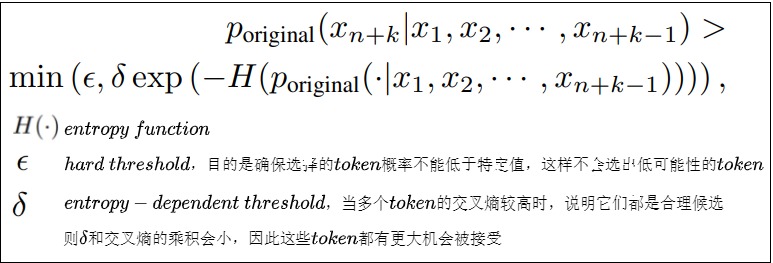
具体实现位于evaluate_posterior()函数中,这里不再赘述。
0x04 训练
MEDUSA的这些分类头需要经过训练才能有比较好的预测效果。针对不同的条件,可以选择不同的训练方式:
- MEDUSA-1:冻结原模型的backbone(包括原模型的解码头),只训练增加的解码头。这种方案适用于计算资源比较少,或者不想影响原模型的效果的情况。还可以使用QLoRA对解码头进行训练,进一步节省内存和计算资源。
- MEDUSA-2:原模型和MEDUSA的解码头一起训练。MEDUSA-1这样的训练方法虽然可以节省资源,但是并不能最大程度发挥多个解码头的加速效果,而MEDUSA-2则可以进一步发挥MEDUSA解码头的提速能力。而且,由于是基干模型与Medusa Heads一起进行训练,确保了MEDUSA heads的分布与原始模型的分布保持一致,从而减轻了分布漂移问题,显著提高Heads的准确性。MEDUSA-2适用于计算资源充足,或者从Base模型进行SFT的场景。
另外,如果原模型的SFT数据集是available的,那可以直接进行训练。如果不能获得原模型的SFT数据,或者原模型是经过RLHF训练的,则可以通过self-distillation来获取MEDUSA head的训练数据。
4.1 MEDUSA-1
MEDUSA-1冻结了原模型的参数,而只对新增的解码头进行训练。使用Medusa-1训练Heads,主要计算Medusa Heads预测的结果与Ground Truth之间的交叉熵损失。具体计算为,给定位置 t+k+1 处的Ground Truth \(y_{t+k+1}\) ,则第 k 个Head的训练loss可以写作:
\\\mathcal{L}_k=-\\log p_t\^{(k)}(y_{t+k+1}) \\
并且当k 较大时, \(\mathcal{L}_k\) 也会随之变大,因为当 k 变大时,靠后的Head的预测将更加不确定。为了平衡各个 Head 上 loss 的大小,因此在 \(\mathcal{L}_k\) 上增加指数衰减的权重参数 \(\lambda_k\) 来平衡不同head的损失。最终Medusa的损失计算如下:
\\\mathcal{L}_{\\text{MEDUSA-l}}=\\sum_{k=1}\^K-\\lambda_k\\log p_t\^{(k)}(y_{t+k+1}) \\
这里的 \(\lambda_{k}\) 是每个解码头的缩放系数,是一系列超参。因为 k 越大,对应解码头的预测难度越大,loss也就越大,为了防止靠后的解码头过分主导训练,因此使用一个缩放系数进行调整。实际使用中,\(\lambda_{k}=0.8^{k}\)。
4.2 MEDUSA-2
为了进一步提高Medusa Heads的准确性,MEDUSA-2把原模型和多个解码头一起训练,因此各个解码头的准确率能达到更高的水平,acceleration rate也更高。但是为了保持原模型的输出质量,需要一些特殊的训练技巧。Medusa-2使用以下三个策略来实现这个目标。
Combined loss
为了保持backbone模型 next token预测的能力,需要将backbone模型的交叉熵损失 \(L_{LM}\)添加到Medusa损失中,即把原模型解码头的loss也加上。同时还需要添加一个权重因子 \(\lambda_0\) 来平衡backbone和Medusa Heads之间的损失。具体如下式
\\\mathcal{L}_{\\text{MEDUSA-}2}=\\mathcal{L}_{\\text{LM}}+\\lambda_0\\mathcal{L}_{\\text{MEDUSA-}1} \\\\\\mathcal{L}_{\\text{LM}}=-\\log p_t\^{(0)}(y_{t+1}) \\
实际使用中,直接训练时 \(\lambda_0=0.2\),使用self-distillation时\(\lambda_0=0.01\)。
Differential learning rates
原模型已经是训练好了的,,而 MEDUSA heads需要更多训练,因此原模型和新加入的解码头使用相同的学习率并不合适。我们可以让新的解码头使用更大的学习率,而原模型参数使用相对小的学习率,以实现 MEDUSA heads更快的收敛,同时保留backbone模型的能力。实践中把学习率差距设为4倍,比如分别使用2e-3和5e-4。
Heads warmup
新加入的解码头在一开始训练会有比较大的loss,从而导致更大的梯度,有可能损害原模型的能力。针对这个问题,可以使用两阶段训练过程g的方式。在第一阶段,先在MEDUSA-1的策略下仅训练解码头,在第二阶段,再进行MEDUSA-2的训练。这其实相当于把 \(\lambda_0\) 在训练过程中逐渐增大。
4.3 代码
我们再来看看一个已经训练好的LLM如何适配MEDUSA,具体分为如下几步:
- 添加解码头:在 LLM 最后一个隐藏层后添加若干个 MEDUSA 解码头。
- 初始化解码头:可使用随机初始化,也可使用原始模型解码头的参数进行初始化,这样可以加快训练速度。
- 选择训练策略 :根据实际情况选择 MEDUSA-1 或 MEDUSA-2 策略。
- 准备训练数据 :可以复用原始模型的训练数据,也可以使用自蒸馏方法生成训练数据。
- 训练 :根据选择的策略和数据,训练 MEDUSA 解码头或同时微调 LLM。
训练具体代码如下。首先需要训练几个新增的头,不同的头预测的label的偏移量不同,所以可以组装每个头的topk作为候选。
python
# Customized for training Medusa heads
class CustomizedTrainer(Trainer):
    def compute_loss(self, model, inputs, return_outputs=False):
        """
        Compute the training loss for the model.

        Args:
            model (torch.nn.Module): The model for which to compute the loss.
            inputs (dict): The input data, including input IDs, attention mask, and labels.
            return_outputs (bool): Whether to return model outputs along with the loss.

        Returns:
            Union[float, Tuple[float, torch.Tensor]]: The computed loss, optionally with model outputs.
        """
        # DDP will give us model.module
        if hasattr(model, "module"):
            medusa = model.module.medusa
        else:
            medusa = model.medusa

        logits = model(
            input_ids=inputs["input_ids"], attention_mask=inputs["attention_mask"]
        )
        labels = inputs["labels"]
        # Shift so that tokens < n predict n
        loss = 0
        loss_fct = CrossEntropyLoss()
        log = {}
        for i in range(medusa):
            medusa_logits = logits[i, :, : -(2 + i)].contiguous()
            # 常规的标签需要偏移1个位置, 由于不训练LM Head,所以偏移2个位置.
            medusa_labels = labels[..., 2 + i :].contiguous()
            medusa_logits = medusa_logits.view(-1, logits.shape[-1])
            medusa_labels = medusa_labels.view(-1)
            medusa_labels = medusa_labels.to(medusa_logits.device)
            loss_i = loss_fct(medusa_logits, medusa_labels)
            loss += loss_i
            not_ignore = medusa_labels.ne(IGNORE_TOKEN_ID)
            medusa_labels = medusa_labels[not_ignore]

            # Add top-k accuracy
            for k in range(1, 2):
                _, topk = medusa_logits.topk(k, dim=-1)
                topk = topk[not_ignore]
                correct = topk.eq(medusa_labels.unsqueeze(-1)).any(-1)

        return (loss, logits) if return_outputs else loss
0x05 Decoding
5.1 示例
官方github源码给出了前向传播代码如下。
python
@contextmanager
def timed(wall_times, key):
    start = time.time()
    torch.cuda.synchronize()
    yield
    torch.cuda.synchronize()
    end = time.time()
    elapsed_time = end - start
    wall_times[key].append(elapsed_time)

def medusa_forward(input_ids, model, tokenizer, medusa_choices, temperature, posterior_threshold, posterior_alpha, max_steps = 512):
    wall_times = {'medusa': [], 'tree': [], 'posterior': [], 'update': [], 'init': []}

    with timed(wall_times, 'init'):
        if hasattr(model, "medusa_choices") and model.medusa_choices == medusa_choices:
            # Load the cached medusa buffer
            medusa_buffers = model.medusa_buffers
        else:
            # Initialize the medusa buffer
            medusa_buffers = generate_medusa_buffers(
                medusa_choices, device=model.base_model.device
            )
        model.medusa_buffers = medusa_buffers
        model.medusa_choices = medusa_choices

        # Initialize the past key and value states
        if hasattr(model, "past_key_values"):
            past_key_values = model.past_key_values
            past_key_values_data = model.past_key_values_data
            current_length_data = model.current_length_data
            # Reset the past key and value states
            current_length_data.zero_()
        else:
            (
                past_key_values,
                past_key_values_data,
                current_length_data,
            ) = initialize_past_key_values(model.base_model)
            model.past_key_values = past_key_values
            model.past_key_values_data = past_key_values_data
            model.current_length_data = current_length_data

        input_len = input_ids.shape[1]
        reset_medusa_mode(model)
        medusa_logits, logits = initialize_medusa(
                input_ids, model, medusa_buffers["medusa_attn_mask"], past_key_values
        )
    new_token = 0

    for idx in range(max_steps):
        with timed(wall_times, 'medusa'):
            candidates, tree_candidates = generate_candidates(
                    medusa_logits,
                    logits,
                    medusa_buffers["tree_indices"],
                    medusa_buffers["retrieve_indices"],
                )

        with timed(wall_times, 'tree'):
            medusa_logits, logits, outputs = tree_decoding(
                    model,
                    tree_candidates,
                    past_key_values,
                    medusa_buffers["medusa_position_ids"],
                    input_ids,
                    medusa_buffers["retrieve_indices"],
                )

        with timed(wall_times, 'posterior'):
            best_candidate, accept_length = evaluate_posterior(
                    logits, candidates, temperature, posterior_threshold, posterior_alpha
                )

        with timed(wall_times, 'update'):
            input_ids, logits, medusa_logits, new_token = update_inference_inputs(
                    input_ids,
                    candidates,
                    best_candidate,
                    accept_length,
                    medusa_buffers["retrieve_indices"],
                    outputs,
                    logits,
                    medusa_logits,
                    new_token,
                    past_key_values_data,
                    current_length_data,
                )

        if tokenizer.eos_token_id in input_ids[0, input_len:].tolist():
            break

    return input_ids, new_token, idx, wall_times
调用方法样例如下。
python
import os
os.environ["CUDA_VISIBLE_DEVICES"] = "3" # define GPU id, remove if you want to use all GPUs available
import torch
from tqdm import tqdm
import time
from contextlib import contextmanager
import numpy as np
from medusa.model.modeling_llama_kv import LlamaForCausalLM as KVLlamaForCausalLM
from medusa.model.medusa_model import MedusaModel
from medusa.model.kv_cache import *
from medusa.model.utils import *
from medusa.model.medusa_choices import *
import transformers
from huggingface_hub import hf_hub_download

# 加载模型
model_name = 'FasterDecoding/medusa-vicuna-7b-v1.3'
model = MedusaModel.from_pretrained(
    model_name,
    medusa_num_heads = 4,
    torch_dtype=torch.float16,
    low_cpu_mem_usage=True,
    device_map="auto"
)
tokenizer = model.get_tokenizer()

medusa_choices = mc_sim_7b_63

# 设置推理参数
temperature = 0.
posterior_threshold = 0.09
posterior_alpha = 0.3

# 设置prompt
prompt = "A chat between a curious user and an artificial intelligence assistant. The assistant gives helpful, detailed, and polite answers to the user's questions. USER: Hi, could you share a tale about a charming llama that grows Medusa-like hair and starts its own coffee shop? ASSISTANT:"

# 执行推理
with torch.inference_mode():
    input_ids = tokenizer([prompt]).input_ids
    output_ids, new_token, idx, wall_time = medusa_forward(
                    torch.as_tensor(input_ids).cuda(),
                    model,
                    tokenizer,
                    medusa_choices,
                    temperature,
                    posterior_threshold,
                    posterior_alpha,
                )
    output_ids = output_ids[0][len(input_ids[0]) :]
    print("Output length:", output_ids.size(-1))
    print("Compression ratio:", new_token / idx)

# 解码
output = tokenizer.decode(
                    output_ids,
                    spaces_between_special_tokens=False,
                )
print(output)
5.2 计算和空间复杂度
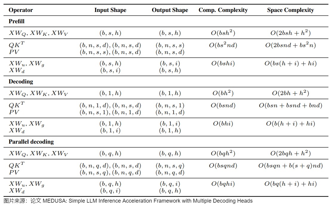
下图给出了prefill,decoding、MEDUSA decoding阶段的计算和空间复杂度。
- b是batch size。
- s是序列长度。
- h是hidden dimension。
- i是intermediate dimension。
- n是注意力头个数。
- d是头维度。
- q是MEDUSA的候选长度。
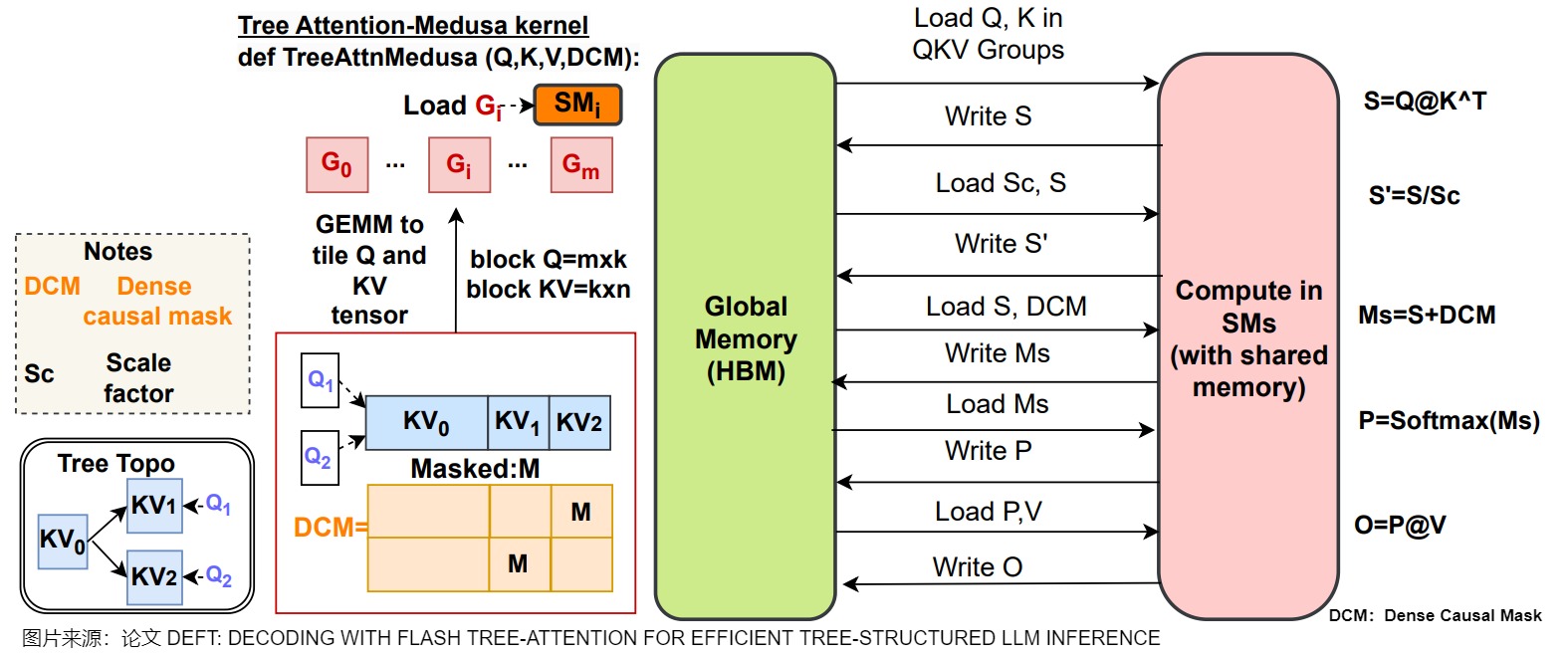
另外,下图给出了Medusa 的操作流程。当没有算子融合或者Tiling策略时,\(QK^⊤\),DCM(Dense Causal Mask),Softmax都会导致显存和片上缓存之间大量的IO操作。
0xFF 参考
Medusa: Simple LLM Inference Acceleration Framework with Multiple Decoding Heads
【手撕LLM-Medusa】并行解码范式: 美杜莎驾到, 通通闪开!! 小冬瓜AIGC
方佳瑞:大模型推理妙招---投机采样(Speculative Decoding)
Transformer 101系列 深入LLM投机采样(上) aaronxic
https://github.com/FasterDecoding/Medusa/blob/main/notebooks/medusa_introduction.ipynb
Medusa: Simple LLM Inference Acceleration Framework with Multiple Decoding Heads, Jan 2024, Princeton University. Proceedings of the ICML 2024.
2401.10774 Medusa: Simple LLM Inference Acceleration Framework with Multiple Decoding Heads
Medusa: Simple LLM Inference Acceleration Framework with Multiple Decoding Heads
LLM推理加速之Medusa:Blockwise Parallel Decoding的继承与发展 方佳瑞
方佳瑞:LLM推理加速的文艺复兴:Noam Shazeer和Blockwise Parallel Decoding?
万字综述 10+ 种 LLM 投机采样推理加速方案 AI闲谈
2401.07851 Unlocking Efficiency in Large Language Model Inference: A Comprehensive Survey of Speculative Decoding
开源进展 | Medusa: 使用多头解码,将大模型推理速度提升2倍以上 洪洗象
arXiv:1811.03115: Berkey, Google Brain, Blockwise Parallel Decoding for Deep Autoregressive Models.
arXiv:2211.17192: Google Research, Fast Inference from Transformers via Speculative Decoding
arXiv:2202.00666: ETH Zürich、University of Cambridge,Locally Typical Sampling
4 arXiv:2106.05234: Dalian University of Technology、Princeton University、Peking University、Microsoft Research Asia,Do Transformers Really Perform Bad for Graph Representation?
3万字详细解析清华大学最新综述工作:大模型高效推理综述 zenRRan
LLM推理加速-Medusa uuuuu
【手撕LLM-Medusa】并行解码范式: 美杜莎驾到, 通通闪开!! 小冬瓜AIGC
Blockwise Parallel Decoding 论文解读 AI闲谈
https://sites.google.com/view/medusa-llm
https://github.com/FasterDecoding/Medusa
百川 Clover:优于 Medusa 的投机采样 AI闲谈
2405.00263 Clover: Regressive Lightweight Speculative Decoding with Sequential Knowledge
Hydra: Sequentially-Dependent Draft Heads for Medusa Decoding 灰瞳六分仪
Hydra: Sequentially-Dependent Draft Heads for Medusa Decoding
【论文解读】Medusa:使用多个解码头并行预测后续多个token tomsheep