1.VGG16背景介绍
VGG16是由牛津大学Visual Geometry Group(VGG)在2014年提出的深度卷积神经网络模型,它在当年的ImageNet图像分类竞赛中取得了优异成绩。
VGG16的主要贡献在于展示了网络深度(层数)对模型性能的重要性,通过使用多个小尺寸(3×3)卷积核堆叠来代替大尺寸卷积核,在保持相同感受野的同时减少了参数数量,提高了模型的非线性表达能力。
VGG16之所以著名,是因为它结构简洁规整,全部使用3×3小卷积核和2×2最大池化层,这种设计理念对后续的CNN架构设计产生了深远影响。
虽然现在有更先进的网络架构(如ResNet、EfficientNet等),但VGG16仍然是理解CNN基础架构的经典案例。
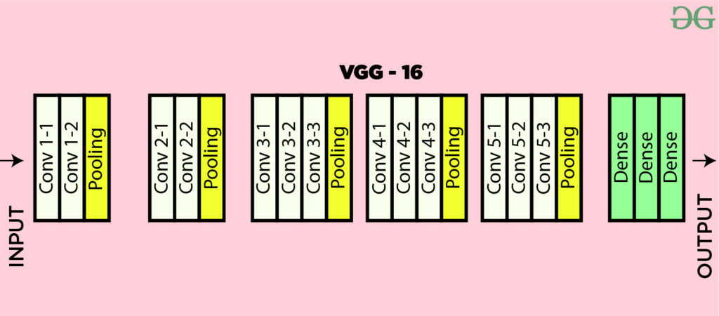
2. VGG16架构详解
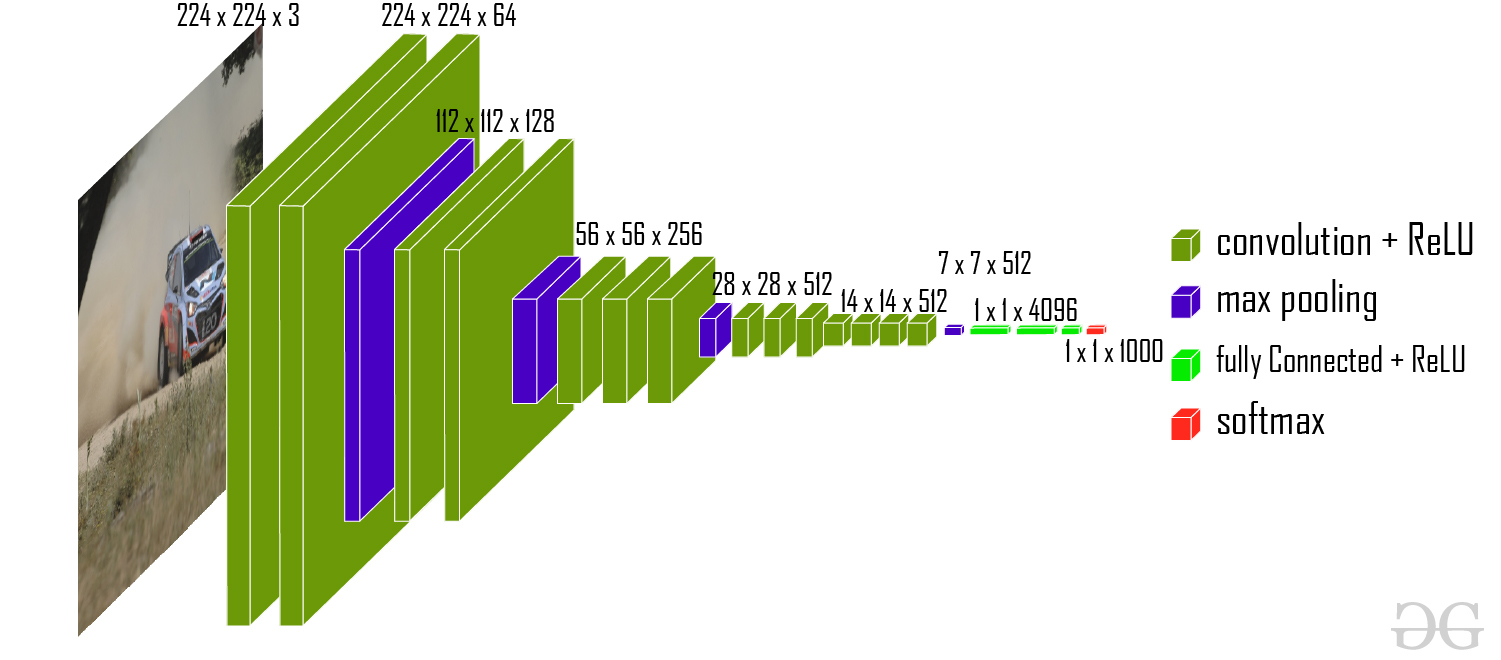
VGG16的架构可以分为两大部分:卷积层部分和全连接层部分。
2.1 卷积层部分
VGG16包含5个卷积块(block),每个块后接一个最大池化层:
- Block1: 2个卷积层(64通道) + 最大池化层
- Block2: 2个卷积层(128通道) + 最大池化层
- Block3: 3个卷积层(256通道) + 最大池化层
- Block4: 3个卷积层(512通道) + 最大池化层
- Block5: 3个卷积层(512通道) + 最大池化层
所有卷积层都使用3×3卷积核,padding=1保持空间尺寸不变,池化层使用2×2窗口,stride=2使尺寸减半。
2.2 全连接层部分
卷积部分后接3个全连接层:
- 第一个全连接层:4096个神经元
- 第二个全连接层:4096个神经元
- 第三个全连接层(输出层):1000个神经元(对应ImageNet的1000类)
在本文的代码实现中,我们将其调整为10个输出神经元,以适应FashionMNIST数据集的10分类任务。
3. 每层参数计算详解
理解CNN的参数计算对于掌握模型复杂度至关重要。我们以VGG16为例详细说明:
3.1 卷积层参数计算
卷积层的参数数量计算公式为:
参数数量 = (输入通道数 × 卷积核宽度 × 卷积核高度 + 1) × 输出通道数
以第一个卷积层为例:
- 输入通道:1(灰度图)
- 卷积核:3×3
- 输出通道:64
- 参数数量 = (1×3×3+1)×64 = 640
3.2 全连接层参数计算
全连接层的参数数量计算公式为:
参数数量 = (输入特征数 + 1) × 输出特征数
以第一个全连接层为例:
- 输入特征数:512×7×7=25088(最后一个卷积层输出512通道,7×7空间尺寸)
- 输出特征数:4096
- 参数数量 = (25088+1)×4096 ≈ 102.7M
3.3 VGG16总参数
VGG16的总参数约为1.38亿,其中大部分参数集中在全连接层。这也是为什么后来的网络架构(如ResNet)倾向于使用全局平均池化代替全连接层来减少参数数量。
4. 代码详解
4.1 模型定义(models.py)
import os  # 导入os模块,用于操作系统相关功能
import sys  # 导入sys模块,用于操作Python运行环境

sys.path.append(os.getcwd())  # 将当前工作目录添加到sys.path,方便模块导入

import torch  # 导入PyTorch主库
from torch import nn  # 从torch中导入神经网络模块
from torchsummary import summary  # 导入模型结构摘要工具


class VGG16(nn.Module):  # 定义VGG16模型,继承自nn.Module
    def __init__(self, *args, **kwargs):  # 构造函数
        super().__init__(*args, **kwargs)  # 调用父类构造函数
        self.block1 = nn.Sequential(  # 第一块卷积层
            nn.Conv2d(
                in_channels=1, out_channels=64, kernel_size=3, padding=1
            ),  # 卷积层,输入通道1,输出通道64
            nn.ReLU(),  # 激活函数
            nn.Conv2d(
                in_channels=64, out_channels=64, kernel_size=3, padding=1
            ),  # 卷积层
            nn.ReLU(),  # 激活函数
            nn.MaxPool2d(kernel_size=2, stride=2),  # 最大池化层
        )

        self.block2 = nn.Sequential(  # 第二块卷积层
            nn.Conv2d(
                in_channels=64, out_channels=128, kernel_size=3, padding=1
            ),  # 卷积层
            nn.ReLU(),  # 激活函数
            nn.Conv2d(
                in_channels=128, out_channels=128, kernel_size=3, padding=1
            ),  # 卷积层
            nn.ReLU(),  # 激活函数
            nn.MaxPool2d(kernel_size=2, stride=2),  # 最大池化层
        )

        self.block3 = nn.Sequential(  # 第三块卷积层
            nn.Conv2d(
                in_channels=128, out_channels=256, kernel_size=3, padding=1
            ),  # 卷积层
            nn.ReLU(),  # 激活函数
            nn.Conv2d(
                in_channels=256, out_channels=256, kernel_size=3, padding=1
            ),  # 卷积层
            nn.ReLU(),  # 激活函数
            nn.Conv2d(
                in_channels=256, out_channels=256, kernel_size=3, padding=1
            ),  # 卷积层
            nn.ReLU(),  # 激活函数
            nn.MaxPool2d(kernel_size=2, stride=2),  # 最大池化层
        )

        self.block4 = nn.Sequential(  # 第四块卷积层
            nn.Conv2d(
                in_channels=256, out_channels=512, kernel_size=3, padding=1
            ),  # 卷积层
            nn.ReLU(),  # 激活函数
            nn.Conv2d(
                in_channels=512, out_channels=512, kernel_size=3, padding=1
            ),  # 卷积层
            nn.ReLU(),  # 激活函数
            nn.Conv2d(
                in_channels=512, out_channels=512, kernel_size=3, padding=1
            ),  # 卷积层
            nn.ReLU(),  # 激活函数
            nn.MaxPool2d(kernel_size=2, stride=2),  # 最大池化层
        )

        self.block5 = nn.Sequential(  # 第五块卷积层
            nn.Conv2d(
                in_channels=512, out_channels=512, kernel_size=3, padding=1
            ),  # 卷积层
            nn.ReLU(),  # 激活函数
            nn.Conv2d(
                in_channels=512, out_channels=512, kernel_size=3, padding=1
            ),  # 卷积层
            nn.ReLU(),  # 激活函数
            nn.Conv2d(
                in_channels=512, out_channels=512, kernel_size=3, padding=1
            ),  # 卷积层
            nn.ReLU(),  # 激活函数
            nn.MaxPool2d(kernel_size=2, stride=2),  # 最大池化层
        )

        self.block6 = nn.Sequential(  # 全连接层部分
            nn.Flatten(),  # 展平多维输入为一维
            nn.Linear(in_features=512 * 7 * 7, out_features=4096),  # 全连接层
            nn.ReLU(),  # 激活函数
            nn.Dropout(p=0.5),  # Dropout防止过拟合
            nn.Linear(in_features=4096, out_features=4096),  # 全连接层
            nn.ReLU(),  # 激活函数
            nn.Dropout(p=0.5),  # Dropout防止过拟合
            nn.Linear(4096, 10),  # 输出层,10分类
        )

        for m in self.modules():  # 遍历所有子模块
            print(m)  # 打印模块信息
            if isinstance(m, nn.Conv2d):  # 如果是卷积层
                nn.init.kaiming_normal_(
                    m.weight, mode="fan_out", nonlinearity="relu"
                )  # 使用Kaiming初始化权重

                if m.bias is not None:  # 如果有偏置
                    nn.init.constant_(m.bias, 0)  # 偏置初始化为0

            if isinstance(m, nn.Linear):  # 如果是全连接层
                nn.init.normal_(m.weight, 0, 0.01)  # 权重正态分布初始化

    def forward(self, x):  # 前向传播
        x = self.block1(x)  # 经过第一块
        x = self.block2(x)  # 经过第二块
        x = self.block3(x)  # 经过第三块
        x = self.block4(x)  # 经过第四块
        x = self.block5(x)  # 经过第五块
        x = self.block6(x)  # 经过全连接层

        return x  # 返回输出


if __name__ == "__main__":  # 脚本主入口
    device = torch.device("cuda" if torch.cuda.is_available() else "cpu")  # 选择设备

    model = VGG16().to(device=device)  # 实例化模型并移动到设备

    print(model)  # 打印模型结构
    summary(model, input_size=(1, 224, 224), device=str(device))  # 打印模型摘要
4.2 训练代码(train.py)
import os
import sys

sys.path.append(os.getcwd())  # 添加上级目录到系统路径中,以便导入自定义模块

import time  # 导入time模块,用于计时训练过程
from torchvision.datasets import FashionMNIST  # 导入FashionMNIST数据集类
from torchvision import transforms  # 导入transforms模块,用于对图像进行预处理
from torch.utils.data import (
    DataLoader,
    random_split,
)  # 导入DataLoader用于批量加载数据,random_split用于划分数据集
import numpy as np  # 导入numpy库,常用于数值计算
import matplotlib.pyplot as plt  # 导入matplotlib的pyplot模块,用于绘图
import torch  # 导入PyTorch主库
from torch import nn, optim  # 从torch中导入神经网络模块和优化器模块
import copy  # 导入copy模块,用于深拷贝模型参数
import pandas as pd  # 导入pandas库,用于数据处理和分析

from VGG16_model.model import VGG16


def train_val_date_load():
    # 加载FashionMNIST训练集,并进行必要的预处理
    train_dataset = FashionMNIST(
        root="./data",  # 数据集存储路径
        train=True,  # 指定加载训练集
        download=True,  # 如果本地没有数据则自动下载
        transform=transforms.Compose(
            [
                transforms.Resize(size=224),
                transforms.ToTensor(),
            ]
        ),
    )

    # 按照8:2的比例将训练集划分为新的训练集和验证集
    train_date, val_data = random_split(
        train_dataset,
        [
            int(len(train_dataset) * 0.8),  # 80%作为训练集
            len(train_dataset) - int(len(train_dataset) * 0.8),  # 剩余20%作为验证集
        ],
    )

    # 构建训练集的数据加载器,设置批量大小为128,打乱数据,使用8个子进程加载数据
    train_loader = DataLoader(
        dataset=train_date, batch_size=16, shuffle=True, num_workers=1
    )

    # 构建验证集的数据加载器,设置批量大小为128,打乱数据,使用8个子进程加载数据
    val_loader = DataLoader(
        dataset=val_data, batch_size=16, shuffle=True, num_workers=1
    )

    return train_loader, val_loader  # 返回训练集和验证集的数据加载器


def train_model_process(model, train_loader, val_loader, epochs=10):
    # 训练模型的主流程,包含训练和验证过程
    device = (
        "cuda" if torch.cuda.is_available() else "cpu"
    )  # 判断是否有GPU可用,否则使用CPU
    optimizer = optim.Adam(
        model.parameters(), lr=0.001
    )  # 使用Adam优化器,学习率为0.001
    criterion = nn.CrossEntropyLoss()  # 使用交叉熵损失函数
    model.to(device)  # 将模型移动到指定设备上

    best_model_wts = copy.deepcopy(model.state_dict())  # 保存最佳模型参数的副本
    best_acc = 0.0  # 初始化最佳验证准确率
    train_loss_all = []  # 用于记录每轮训练损失
    val_loss_all = []  # 用于记录每轮验证损失
    train_acc_all = []  # 用于记录每轮训练准确率
    val_acc_all = []  # 用于记录每轮验证准确率

    since = time.time()  # 记录训练开始时间

    for epoch in range(epochs):  # 遍历每一个训练轮次
        print(f"Epoch {epoch + 1}/{epochs}")  # 打印当前轮次信息

        train_loss = 0.0  # 当前轮训练损失总和
        train_correct = 0  # 当前轮训练正确样本数

        val_loss = 0.0  # 当前轮验证损失总和
        val_correct = 0  # 当前轮验证正确样本数

        train_num = 0  # 当前轮训练样本总数
        val_num = 0  # 当前轮验证样本总数

        for step, (images, labels) in enumerate(train_loader):  # 遍历训练集的每个批次
            images = images.to(device)  # 将图片数据移动到设备上
            labels = labels.to(device)  # 将标签数据移动到设备上

            model.train()  # 设置模型为训练模式

            outputs = model(images)  # 前向传播,得到模型输出

            pre_lab = torch.argmax(outputs, dim=1)  # 获取预测的类别标签

            loss = criterion(outputs, labels)  # 计算损失值

            optimizer.zero_grad()  # 梯度清零
            loss.backward()  # 反向传播计算梯度
            optimizer.step()  # 更新模型参数

            train_loss += loss.item() * images.size(0)  # 累加当前批次的损失
            train_correct += torch.sum(
                pre_lab == labels.data
            )  # 累加当前批次预测正确的样本数
            train_num += labels.size(0)  # 累加当前批次的样本数

            print(
                "Epoch [{}/{}], Step [{}/{}], Loss: {:.4f}, Acc:{:.4f}".format(
                    epoch + 1,
                    epochs,
                    step + 1,
                    len(train_loader),
                    loss.item(),
                    torch.sum(pre_lab == labels.data),
                )
            )

        for step, (images, labels) in enumerate(val_loader):  # 遍历验证集的每个批次
            images = images.to(device)  # 将图片数据移动到设备上
            labels = labels.to(device)  # 将标签数据移动到设备上
            model.eval()  # 设置模型为评估模式

            with torch.no_grad():  # 关闭梯度计算,提高验证速度,节省显存
                outputs = model(images)  # 前向传播,得到模型输出
                pre_lab = torch.argmax(outputs, dim=1)  # 获取预测的类别标签
                loss = criterion(outputs, labels)  # 计算损失值

                val_loss += loss.item() * images.size(0)  # 累加当前批次的损失
                val_correct += torch.sum(
                    pre_lab == labels.data
                )  # 累加当前批次预测正确的样本数
                val_num += labels.size(0)  # 累加当前批次的样本数

                print(
                    "Epoch [{/{}], Step [{}/{}], Val Loss: {:.4f}, Acc:{:.4f}".format(
                        epoch + 1,
                        epochs,
                        step + 1,
                        len(val_loader),
                        loss.item(),
                        torch.sum(pre_lab == labels.data),
                    )
                )

        train_loss_all.append(train_loss / train_num)  # 记录当前轮的平均训练损失
        val_loss_all.append(val_loss / val_num)  # 记录当前轮的平均验证损失
        train_acc = train_correct.double() / train_num  # 计算当前轮的训练准确率
        val_acc = val_correct.double() / val_num  # 计算当前轮的验证准确率
        train_acc_all.append(train_acc.item())  # 记录当前轮的训练准确率
        val_acc_all.append(val_acc.item())  # 记录当前轮的验证准确率
        print(
            f"Train Loss: {train_loss / train_num:.4f}, Train Acc: {train_acc:.4f}, "
            f"Val Loss: {val_loss / val_num:.4f}, Val Acc: {val_acc:.4f}"
        )  # 打印当前轮的损失和准确率
        if val_acc_all[-1] > best_acc:  # 如果当前验证准确率优于历史最佳
            best_acc = val_acc_all[-1]  # 更新最佳准确率
            best_model_wts = copy.deepcopy(model.state_dict())  # 保存当前最佳模型参数

        # model.load_state_dict(best_model_wts)  # 可选:恢复最佳模型参数

    time_elapsed = time.time() - since  # 计算训练总耗时
    print(
        f"Training complete in {time_elapsed // 60:.0f}m {time_elapsed % 60:.0f}s\n"
        f"Best val Acc: {best_acc:.4f}"
    )  # 打印训练完成信息和最佳验证准确率

    torch.save(
        model.state_dict(), "./models/vgg16_net_best_model.pth"
    )  # 保存最终模型参数到文件
    train_process = pd.DataFrame(
        data={
            "epoch": range(1, epochs + 1),  # 轮次编号
            "train_loss_all": train_loss_all,  # 每轮训练损失
            "val_loss_all": val_loss_all,  # 每轮验证损失
            "train_acc_all": train_acc_all,  # 每轮训练准确率
            "val_acc_all": val_acc_all,  # 每轮验证准确率
        }
    )

    return train_process  # 返回训练过程的详细数据


def matplot_acc_loss(train_process):
    # 绘制训练和验证的损失及准确率曲线
    plt.figure(figsize=(12, 5))  # 创建一个宽12高5的画布

    plt.subplot(1, 2, 1)  # 创建1行2列的子图,激活第1个
    plt.plot(
        train_process["epoch"], train_process["train_loss_all"], label="Train Loss"
    )  # 绘制训练损失曲线
    plt.plot(
        train_process["epoch"], train_process["val_loss_all"], label="Val Loss"
    )  # 绘制验证损失曲线
    plt.xlabel("Epoch")  # 设置x轴标签为Epoch
    plt.ylabel("Loss")  # 设置y轴标签为Loss
    plt.title("Loss vs Epoch")  # 设置子图标题
    plt.legend()  # 显示图例

    plt.subplot(1, 2, 2)  # 激活第2个子图
    plt.plot(
        train_process["epoch"], train_process["train_acc_all"], label="Train Acc"
    )  # 绘制训练准确率曲线
    plt.plot(
        train_process["epoch"], train_process["val_acc_all"], label="Val Acc"
    )  # 绘制验证准确率曲线
    plt.xlabel("Epoch")  # 设置x轴标签为Epoch
    plt.ylabel("Accuracy")  # 设置y轴标签为Accuracy
    plt.title("Accuracy vs Epoch")  # 设置子图标题
    plt.legend()  # 显示图例

    plt.tight_layout()  # 自动调整子图间距
    plt.ion()  # 关闭交互模式,防止图像自动关闭
    plt.show()  # 显示所有图像
    plt.savefig("./models/vgg16_net_output.png")


if __name__ == "__main__":  # 如果当前脚本作为主程序运行
    traindatam, valdata = train_val_date_load()  # 加载训练集和验证集
    result = train_model_process(VGG16(), traindatam, valdata, 10)
    matplot_acc_loss(result)  # 绘制训练和验证的损失及准确率曲线
4.3 测试代码(test.py)
import os  # 导入os模块,用于处理文件和目录
import sys

sys.path.append(os.getcwd())  # 添加上级目录到系统路径,以便导入其他模块

import torch
from torch.utils.data import (
    DataLoader,
    random_split,
)
from torchvision import datasets, transforms
from torchvision.datasets import FashionMNIST
from VGG16_model.model import VGG16  # 导入自定义的模型


def test_data_load():
    test_dataset = FashionMNIST(
        root="./data",
        train=False,
        download=True,
        transform=transforms.Compose(
            [
                transforms.Resize(size=224),
                transforms.ToTensor(),
            ]
        ),
    )

    test_loader = DataLoader(
        dataset=test_dataset, batch_size=16, shuffle=True, num_workers=1
    )

    return test_loader


print(test_data_load())


def test_model_process(model, test_loader):
    device = "cuda" if torch.cuda.is_available() else "cpu"
    model.to(device)
    model.eval()  # 设置模型为评估模式

    correct = 0
    total = 0

    with torch.no_grad():  # 在测试时不需要计算梯度
        for images, labels in test_loader:
            images, labels = images.to(device), labels.to(device)
            outputs = model(images)  # 前向传播
            _, predicted = torch.max(outputs, 1)  # 获取预测结果
            total += labels.size(0)  # 累计总样本数
            correct += torch.sum(predicted == labels.data)  # 累计正确预测的样本数

    accuracy = correct / total * 100  # 计算准确率
    print(f"Test Accuracy: {accuracy:.2f}%")  # 打印测试准确率


if __name__ == "__main__":
    test_loader = test_data_load()  # 加载测试数据
    model = VGG16()  # 实例化模型
    model.load_state_dict(
        torch.load("./models/vgg16_net_best_model.pth")
    )  # 加载模型参数
    test_model_process(model, test_loader)  # 进行模型测试
5. 总结
VGG16作为深度学习发展史上的里程碑式模型,其设计理念至今仍有重要参考价值:
-
小卷积核优势:通过堆叠多个3×3小卷积核代替大卷积核,在保持相同感受野的同时减少了参数数量,增加了非线性表达能力。
-
深度重要性:VGG16证明了增加网络深度可以显著提高模型性能,为后续更深网络(如ResNet)的研究奠定了基础。
-
结构规整:VGG16结构简洁规整,便于理解和实现,是学习CNN架构的优秀范例。
-
初始化技巧:代码中展示了Kaiming初始化等现代神经网络训练技巧,这些对于模型收敛至关重要。
-
完整流程:本文提供了从数据加载、模型定义、训练到测试的完整流程,可以作为实际项目的参考模板。
虽然VGG16现在可能不是性能最优的选择,但它仍然是理解CNN基础架构的最佳起点。通过本博客的学习,读者应该能够掌握VGG16的核心思想,并能够将其应用到自己的图像分类任务中。