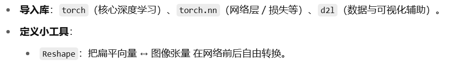
一、导入所用库
python
import torch
from torch import nn
from d2l import torch as d2l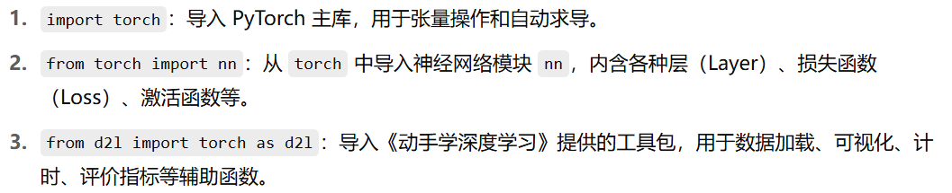
二、自定义重塑层
python
class Reshape(nn.Module):
    def forward(self, x):
        return x.view(-1, 1, 28, 28)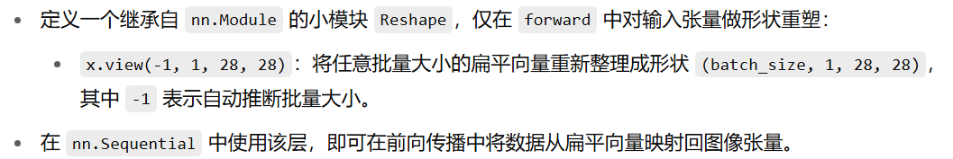
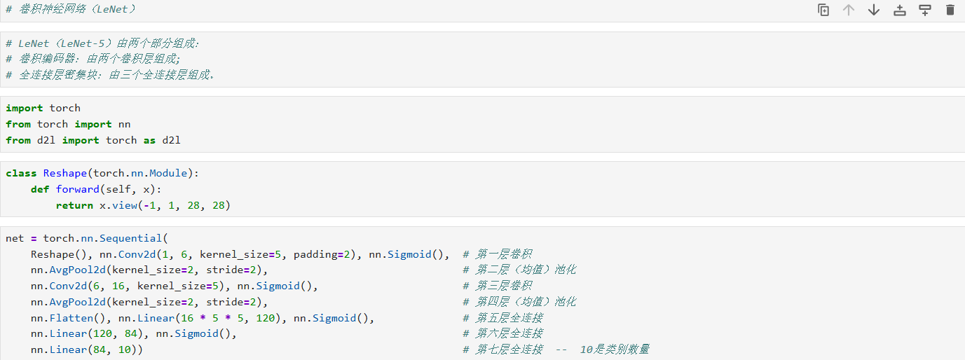
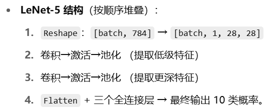
三、构建 LeNet 网络
python
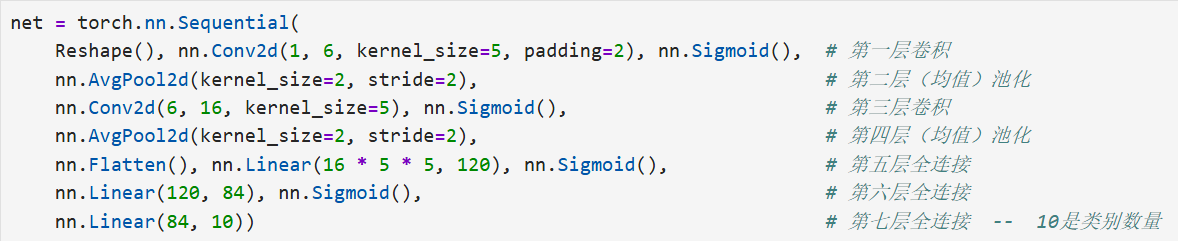
net = nn.Sequential(
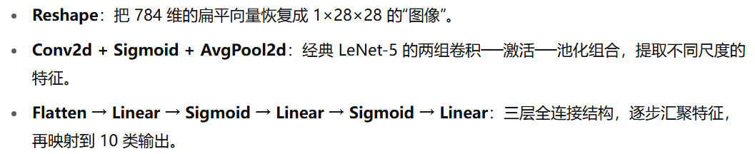
Reshape(), # 将输入 (batch, 784) → (batch, 1, 28, 28)
nn.Conv2d(1, 6, kernel_size=5, padding=2), # 卷积层1:输入通道 1 → 输出通道 6,卷积核 5×5,padding=2 保持宽高不变
nn.Sigmoid(), # 激活函数:Sigmoid
nn.AvgPool2d(kernel_size=2, stride=2), # 平均池化1:kernel=2, stride=2,下采样一半
nn.Conv2d(6, 16, kernel_size=5), # 卷积层2:6→16,kernel=5×5,默认无 padding → 尺寸缩小
nn.Sigmoid(), # Sigmoid 激活
nn.AvgPool2d(kernel_size=2, stride=2), # 平均池化2
nn.Flatten(), # 展平:把多维特征图拉成一维向量
nn.Linear(16 * 5 * 5, 120), # 全连接层1:输入 16×5×5 → 输出 120
nn.Sigmoid(), # Sigmoid 激活
nn.Linear(120, 84), # 全连接层2:120 → 84
nn.Sigmoid(), # Sigmoid 激活
nn.Linear(84, 10) # 输出层:84 → 10 类别
)
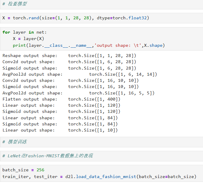
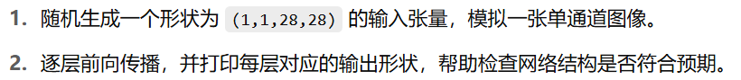
四、验证每层输出形状
python
X = torch.rand(size=(1, 1, 28, 28), dtype=torch.float32)
for layer in net:
    X = layer(X)
    print(layer.__class__.__name__, 'output shape:\t', X.shape)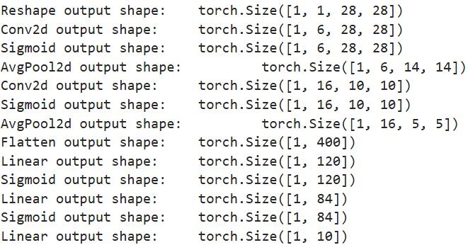
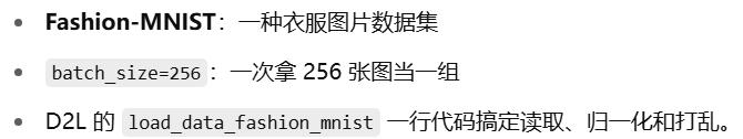
五、加载 Fashion-MNIST 数据
python
batch_size = 256
train_iter, test_iter = d2l.load_data_fashion_mnist(batch_size=batch_size)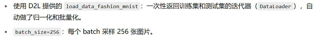
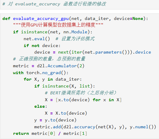
六、定义 GPU 下的准确率评估函数
python
def evaluate_accuracy_gpu(net, data_iter, device=None):
    """在 GPU 上评估模型在给定数据集上的准确率"""
    if isinstance(net, nn.Module):
        net.eval()  # 切换到评估模式,关闭 dropout、batchnorm 等
        if not device:
            device = next(iter(net.parameters())).device
    # metric[0] 累积正确预测数;metric[1] 累积样本总数
    metric = d2l.Accumulator(2)
    with torch.no_grad():
        for X, y in data_iter:
            X, y = X.to(device), y.to(device)
            y_hat = net(X)
            metric.add(d2l.accuracy(y_hat, y), y.numel())
    return metric[0] / metric[1]
七、定义训练函数(带 GPU 支持)
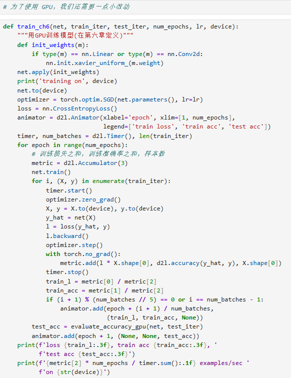
python
def train_ch6(net, train_iter, test_iter, num_epochs, lr, device):
# 1. 权重初始化:对每个线性层和卷积层使用 Xavier 均匀分布初始化
def init_weights(m):
if type(m) in (nn.Linear, nn.Conv2d):
nn.init.xavier_uniform_(m.weight)
net.apply(init_weights)
print('training on', device)
net.to(device) # 把模型参数搬到指定设备
optimizer = torch.optim.SGD(net.parameters(), lr=lr)
loss = nn.CrossEntropyLoss()
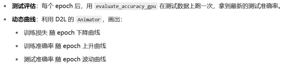
# 可视化工具:训练过程实时画图
animator = d2l.Animator(xlabel='epoch', xlim=[1, num_epochs],
legend=['train loss', 'train acc', 'test acc'])
timer, num_batches = d2l.Timer(), len(train_iter)
# 2. 训练循环
for epoch in range(num_epochs):
# 累积训练损失、训练正确预测数、样本数
metric = d2l.Accumulator(3)
net.train() # 切回训练模式
for i, (X, y) in enumerate(train_iter):
timer.start()
X, y = X.to(device), y.to(device)
optimizer.zero_grad()
y_hat = net(X)
l = loss(y_hat, y)
l.backward()
optimizer.step()
with torch.no_grad():
metric.add(l * y.numel(), d2l.accuracy(y_hat, y), y.numel())
timer.stop()
# 每训练完一个 epoch,或者到达最后一个 batch 时更新可视化
if (i + 1) % (num_batches // 5) == 0 or i == num_batches - 1:
animator.add(epoch + (i + 1) / num_batches,
(metric[0] / metric[2], metric[1] / metric[2], None))
# 每个 epoch 结束后计算一次测试集准确率并更新图示
test_acc = evaluate_accuracy_gpu(net, test_iter, device)
animator.add(epoch + 1, (None, None, test_acc))
# 输出整体训练速度
print(f'{metric[2] * num_epochs / timer.sum():.1f} examples/sec on {device}')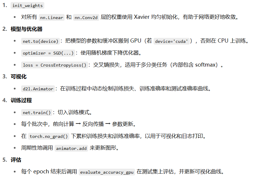
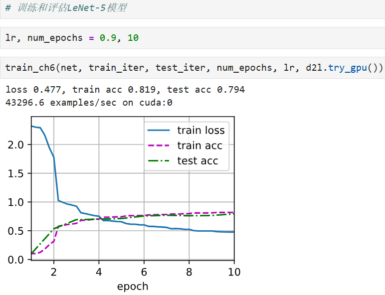
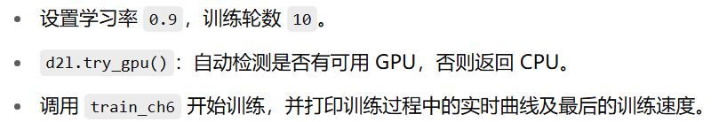
八、运行训练
python
lr, num_epochs = 0.9, 10
train_ch6(net, train_iter, test_iter, num_epochs, lr, d2l.try_gpu())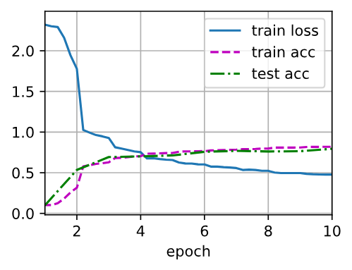
九、总结
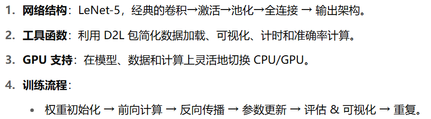
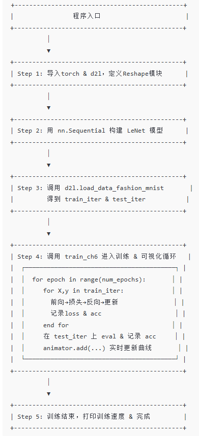
十、流程概览
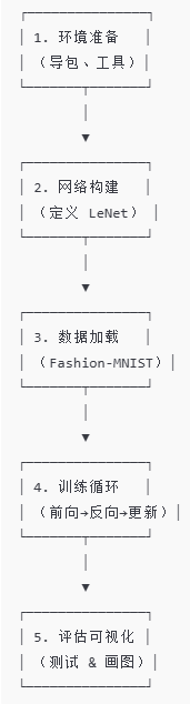
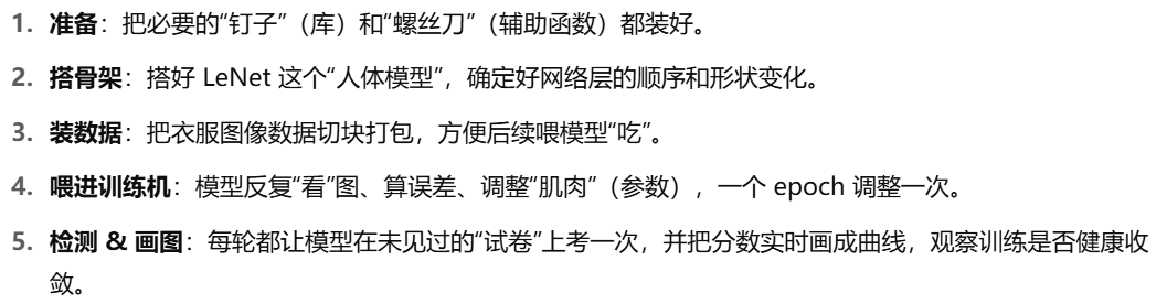
1. 环境准备
2. 网络构建
3. 数据加载
4. 训练循环
python
for epoch in 1...N:
    for 每个 batch (X, y):
        1) 前向计算 ŷ = net(X)
        2) 计算损失 L = Loss(ŷ, y)
        3) 反向传播 L.backward()
        4) 优化器更新参数 optimizer.step()
        5) 累积训练损失 & 正确率
    end-for

    # 每跑完一个 epoch:
    - 在测试集上评估一次准确率
    - 把训练损失、训练准确率、测试准确率推到"动画器"里,实时画图
end-for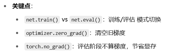
5. 评估与可视化
6. 通俗小结