前言
是看了这个大佬的视频后想进行一下自己的整理(流程只到了扁平化),如果有问题希望各位大佬能够给予指正。卷积神经网络(CNN)到底卷了啥?8分钟带你快速了解!_哔哩哔哩_bilibili![]() https://www.bilibili.com/video/BV1MsrmY4Edi/?spm_id_from=333.1007.top_right_bar_window_history.content.click&vd_source=7c3bfbf39d037fe80c97234396acc524
https://www.bilibili.com/video/BV1MsrmY4Edi/?spm_id_from=333.1007.top_right_bar_window_history.content.click&vd_source=7c3bfbf39d037fe80c97234396acc524
输入层

由于自己也不知道设置什么矩阵,就干脆让deepseek生成0~9的矩阵,每次随机使用一个数字来进行测试。
-
从预定义的
digit_templates中随机选择一个数字(0-9) -
将数字的6x6二进制矩阵转换为NumPy数组
关键变量: -
digit: 原始数字矩阵(6x6),值为0(黑)或1(白)
python
# 数字模板(6x6矩阵)
digit_templates = {
    0: [[0, 1, 1, 1, 1, 0],
        [1, 0, 0, 0, 0, 1],
        [1, 0, 0, 0, 0, 1],
        [1, 0, 0, 0, 0, 1],
        [1, 0, 0, 0, 0, 1],
        [0, 1, 1, 1, 1, 0]],

    1: [[0, 0, 1, 1, 0, 0],
        [0, 1, 1, 1, 0, 0],
        [0, 0, 1, 1, 0, 0],
        [0, 0, 1, 1, 0, 0],
        [0, 0, 1, 1, 0, 0],
        [0, 1, 1, 1, 1, 0]],

    2: [[0, 1, 1, 1, 1, 0],
        [1, 0, 0, 0, 0, 1],
        [0, 0, 0, 1, 1, 0],
        [0, 1, 1, 0, 0, 0],
        [1, 0, 0, 0, 0, 0],
        [1, 1, 1, 1, 1, 1]],

    3: [[1, 1, 1, 1, 1, 0],
        [0, 0, 0, 0, 0, 1],
        [0, 1, 1, 1, 1, 0],
        [0, 0, 0, 0, 0, 1],
        [0, 0, 0, 0, 0, 1],
        [1, 1, 1, 1, 1, 0]],

    4: [[1, 0, 0, 0, 1, 0],
        [1, 0, 0, 0, 1, 0],
        [1, 0, 0, 0, 1, 0],
        [1, 1, 1, 1, 1, 1],
        [0, 0, 0, 0, 1, 0],
        [0, 0, 0, 0, 1, 0]],

    5: [[1, 1, 1, 1, 1, 1],
        [1, 0, 0, 0, 0, 0],
        [1, 1, 1, 1, 1, 0],
        [0, 0, 0, 0, 0, 1],
        [0, 0, 0, 0, 0, 1],
        [1, 1, 1, 1, 1, 0]],

    6: [[0, 1, 1, 1, 1, 0],
        [1, 0, 0, 0, 0, 0],
        [1, 1, 1, 1, 1, 0],
        [1, 0, 0, 0, 0, 1],
        [1, 0, 0, 0, 0, 1],
        [0, 1, 1, 1, 1, 0]],

    7: [[1, 1, 1, 1, 1, 1],
        [0, 0, 0, 0, 1, 0],
        [0, 0, 0, 1, 0, 0],
        [0, 0, 1, 0, 0, 0],
        [0, 1, 0, 0, 0, 0],
        [1, 0, 0, 0, 0, 0]],

    8: [[0, 1, 1, 1, 1, 0],
        [1, 0, 0, 0, 0, 1],
        [0, 1, 1, 1, 1, 0],
        [1, 0, 0, 0, 0, 1],
        [1, 0, 0, 0, 0, 1],
        [0, 1, 1, 1, 1, 0]],

    9: [[0, 1, 1, 1, 1, 0],
        [1, 0, 0, 0, 0, 1],
        [1, 0, 0, 0, 0, 1],
        [0, 1, 1, 1, 1, 1],
        [0, 0, 0, 0, 0, 1],
        [0, 1, 1, 1, 1, 0]]
}

# 随机选择数字
random_digit = randint(0, 9)
digit = np.array(digit_templates[random_digit])
Padding
将6*6的矩阵边界填充0扩展为8x8矩阵,防止丢失边缘信息。
numpy.pad()函数详解_numpy pad-CSDN博客![]() https://blog.csdn.net/weixin_41862755/article/details/128336141
https://blog.csdn.net/weixin_41862755/article/details/128336141
-
在原始矩阵周围添加一圈0(
pad_width=1) -
将6x6矩阵扩展为8x8,防止卷积时边缘信息丢失
输出: -
padded: 填充后的矩阵(8x8)
python
padded = np.pad(digit, pad_width=1, mode='constant') # 边界填充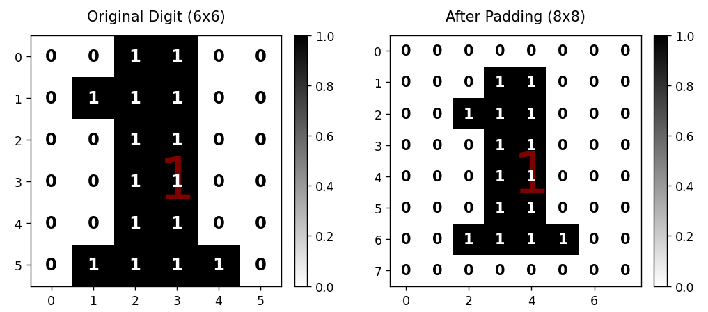
卷积
局部加权求和(对应相乘再相加),提取输入数据的局部特征,形成特征映射。
-
conv2d函数实现滑动窗口卷积运算 -
使用垂直核(
kernel_v)检测垂直边缘特征 -
使用水平核(
kernel_h)检测水平边缘特征
关键参数: -
kernel_v:[[0,1,0], [0,1,0], [0,1,0]](强化垂直线条) -
kernel_h:[[0,0,0], [1,1,1], [0,0,0]](强化水平线条)
输出: -
conv_v: 垂直卷积结果(6x6矩阵) -
conv_h: 水平卷积结果(6x6矩阵)
python
# 定义卷积核
kernel_v = np.array([[0, 1, 0], [0, 1, 0], [0, 1, 0]])  # 垂直特征
kernel_h = np.array([[0, 0, 0], [1, 1, 1], [0, 0, 0]])  # 水平特征

def conv2d(image, kernel):
    # 手动实现卷积运算
    h, w = image.shape
    k_h, k_w = kernel.shape
    output = np.zeros((h - k_h + 1, w - k_w + 1))
    for y in range(h - k_h + 1):
        for x in range(w - k_w + 1):
            output[y, x] = np.sum(image[y:y + k_h, x:x + k_w] * kernel)
    return output.astype(int)

conv_v = conv2d(padded, kernel_v)  # 垂直卷积
conv_h = conv2d(padded, kernel_h)  # 水平卷积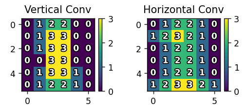
激活
这个视频中没有,然后代码中也没起作用,因为没有出现值为负数出现。激活函数可以进行 非线性变换,使网络能够学习复杂模式,可以进行特征过滤,保留有用特征,抑制噪声,可以优化训练,控制梯度流动,提高模型收敛速度。
-
对卷积结果应用ReLU(Rectified Linear Unit)激活函数
-
保留正值,负值置为0(非线性变换)
输出: -
relu_v: 垂直特征激活结果(6x6) -
relu_h: 水平特征激活结果(6x6)
python
relu_v = np.maximum(0, conv_v)  # ReLU激活
relu_h = np.maximum(0, conv_h)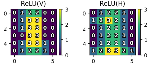
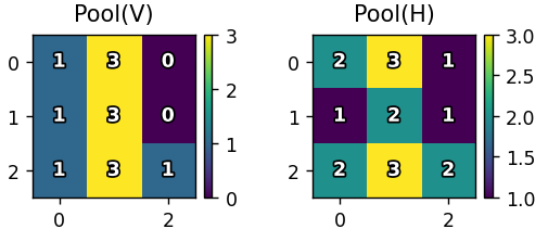
池化
池化能够进行信息压缩,用更少的参数表达关键特征,可以不变性增强,使模型对输入的小变化更鲁棒,可以计算效率,加速训练和推理过程。
-
maxpool2d函数实现2x2最大池化(步长=2) -
降低特征图维度,保留显著特征(保留2*2中的最大值)
输出: -
pool_v: 垂直特征池化结果(3x3) -
pool_h: 水平特征池化结果(3x3)
扁平化
扁平化可以结构转换,让多维特征转换成一维向量,可以信息整合,合并不同特征提取路径的结果,起到桥梁作用,连接特征提取层与分类决策层。
-
将池化后的3x3矩阵展平为一维向量(
flatten()) -
合并垂直和水平特征向量(最终18维向量)
输出: -
flattened: 合并后的特征向量(形状:(18,))
python
flattened = np.concatenate([pool_v.flatten(), pool_h.flatten()])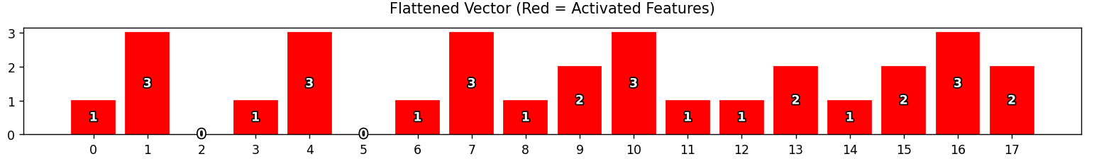
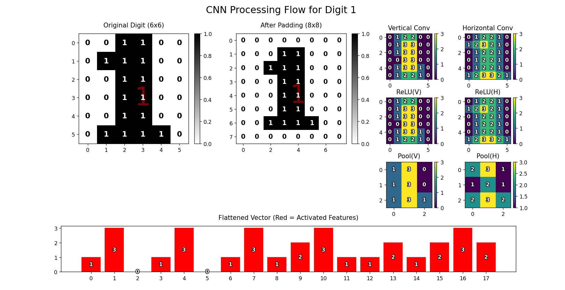
可视化
-
使用Matplotlib绘制处理流程各阶段的结果
-
关键可视化内容:
-
原始数字矩阵(标注0/1值)
-
卷积/激活/池化结果(热力图+数值标注)
-
扁平化向量(条形图,红色标记激活特征)
-
完整代码
python
import numpy as np
import matplotlib.pyplot as plt
import matplotlib.patheffects as path_effects
from random import randint

# 数字模板(6x6矩阵)
digit_templates = {
    0: [[0, 1, 1, 1, 1, 0],
        [1, 0, 0, 0, 0, 1],
        [1, 0, 0, 0, 0, 1],
        [1, 0, 0, 0, 0, 1],
        [1, 0, 0, 0, 0, 1],
        [0, 1, 1, 1, 1, 0]],

    1: [[0, 0, 1, 1, 0, 0],
        [0, 1, 1, 1, 0, 0],
        [0, 0, 1, 1, 0, 0],
        [0, 0, 1, 1, 0, 0],
        [0, 0, 1, 1, 0, 0],
        [0, 1, 1, 1, 1, 0]],

    2: [[0, 1, 1, 1, 1, 0],
        [1, 0, 0, 0, 0, 1],
        [0, 0, 0, 1, 1, 0],
        [0, 1, 1, 0, 0, 0],
        [1, 0, 0, 0, 0, 0],
        [1, 1, 1, 1, 1, 1]],

    3: [[1, 1, 1, 1, 1, 0],
        [0, 0, 0, 0, 0, 1],
        [0, 1, 1, 1, 1, 0],
        [0, 0, 0, 0, 0, 1],
        [0, 0, 0, 0, 0, 1],
        [1, 1, 1, 1, 1, 0]],

    4: [[1, 0, 0, 0, 1, 0],
        [1, 0, 0, 0, 1, 0],
        [1, 0, 0, 0, 1, 0],
        [1, 1, 1, 1, 1, 1],
        [0, 0, 0, 0, 1, 0],
        [0, 0, 0, 0, 1, 0]],

    5: [[1, 1, 1, 1, 1, 1],
        [1, 0, 0, 0, 0, 0],
        [1, 1, 1, 1, 1, 0],
        [0, 0, 0, 0, 0, 1],
        [0, 0, 0, 0, 0, 1],
        [1, 1, 1, 1, 1, 0]],

    6: [[0, 1, 1, 1, 1, 0],
        [1, 0, 0, 0, 0, 0],
        [1, 1, 1, 1, 1, 0],
        [1, 0, 0, 0, 0, 1],
        [1, 0, 0, 0, 0, 1],
        [0, 1, 1, 1, 1, 0]],

    7: [[1, 1, 1, 1, 1, 1],
        [0, 0, 0, 0, 1, 0],
        [0, 0, 0, 1, 0, 0],
        [0, 0, 1, 0, 0, 0],
        [0, 1, 0, 0, 0, 0],
        [1, 0, 0, 0, 0, 0]],

    8: [[0, 1, 1, 1, 1, 0],
        [1, 0, 0, 0, 0, 1],
        [0, 1, 1, 1, 1, 0],
        [1, 0, 0, 0, 0, 1],
        [1, 0, 0, 0, 0, 1],
        [0, 1, 1, 1, 1, 0]],

    9: [[0, 1, 1, 1, 1, 0],
        [1, 0, 0, 0, 0, 1],
        [1, 0, 0, 0, 0, 1],
        [0, 1, 1, 1, 1, 1],
        [0, 0, 0, 0, 0, 1],
        [0, 1, 1, 1, 1, 0]]
}

# 随机选择数字
random_digit = randint(0, 9)
digit = np.array(digit_templates[random_digit])

# 定义卷积核
kernel_v = np.array([[0, 1, 0], [0, 1, 0], [0, 1, 0]])  # 垂直特征
kernel_h = np.array([[0, 0, 0], [1, 1, 1], [0, 0, 0]])  # 水平特征


def process_digit(digit):
    # Padding
    padded = np.pad(digit, pad_width=1, mode='constant')

    # 卷积计算
    def conv2d(image, kernel):
        h, w = image.shape
        k_h, k_w = kernel.shape
        output = np.zeros((h - k_h + 1, w - k_w + 1))
        for y in range(h - k_h + 1):
            for x in range(w - k_w + 1):
                output[y, x] = np.sum(image[y:y + k_h, x:x + k_w] * kernel)
        return output.astype(int)  # 转换为整型

    conv_v = conv2d(padded, kernel_v)
    conv_h = conv2d(padded, kernel_h)

    # ReLU激活
    relu_v = np.maximum(0, conv_v).astype(int)  # 转换为整型
    relu_h = np.maximum(0, conv_h).astype(int)  # 转换为整型

    # 最大池化
    def maxpool2d(image, size=2):
        h, w = image.shape
        return np.array([[np.max(image[i:i + size, j:j + size])
                          for j in range(0, w, size)]
                         for i in range(0, h, size)]).astype(int)  # 转换为整型

    pool_v = maxpool2d(relu_v)
    pool_h = maxpool2d(relu_h)

    # 扁平化
    flattened = np.concatenate([pool_v.flatten(), pool_h.flatten()]).astype(int)  # 转换为整型

    return {
        'original': digit,
        'padded': padded,
        'conv_v': conv_v,
        'conv_h': conv_h,
        'relu_v': relu_v,
        'relu_h': relu_h,
        'pool_v': pool_v,
        'pool_h': pool_h,
        'flattened': flattened
    }


def visualize_flow(results):
    fig = plt.figure(figsize=(20, 12))
    plt.suptitle(f'CNN Processing Flow for Digit {random_digit}', fontsize=18, y=0.97)
    grid = plt.GridSpec(4, 6, hspace=0.4, wspace=0.3)

    # 创建文本描边效果
    text_effect = [path_effects.withStroke(linewidth=2, foreground='black')]

    # 原始图像 - 显示阿拉伯数字
    ax1 = fig.add_subplot(grid[0:2, 0:2])
    img1 = ax1.imshow(results['original'], cmap='binary')
    plt.colorbar(img1, ax=ax1, fraction=0.046, pad=0.04)
    ax1.set_title("Original Digit (6x6)", pad=12)
    ax1.text(3, 3, str(random_digit),
             ha='center', va='center',
             color='red', fontsize=48, alpha=0.5)
    for y in range(results['original'].shape[0]):
        for x in range(results['original'].shape[1]):
            display_val = '1' if results['original'][y, x] > 0.5 else '0'
            ax1.text(x, y, display_val,
                     ha='center', va='center',
                     color='white' if results['original'][y, x] > 0.5 else 'black',
                     fontsize=14, weight='bold')

    # Padding后的图像 - 显示阿拉伯数字
    ax2 = fig.add_subplot(grid[0:2, 2:4])
    img2 = ax2.imshow(results['padded'], cmap='binary')
    plt.colorbar(img2, ax=ax2, fraction=0.046, pad=0.04)
    ax2.set_title("After Padding (8x8)", pad=12)
    ax2.text(4, 4, str(random_digit),
             ha='center', va='center',
             color='red', fontsize=48, alpha=0.5)
    for y in range(results['padded'].shape[0]):
        for x in range(results['padded'].shape[1]):
            display_val = '1' if results['padded'][y, x] > 0.5 else '0'
            ax2.text(x, y, display_val,
                     ha='center', va='center',
                     color='white' if results['padded'][y, x] > 0.5 else 'black',
                     fontsize=12, weight='bold')

    # 右侧图像的统一设置
    right_plots = {
        'conv_v': ('Vertical Conv', grid[0, 4]),
        'conv_h': ('Horizontal Conv', grid[0, 5]),
        'relu_v': ('ReLU(V)', grid[1, 4]),
        'relu_h': ('ReLU(H)', grid[1, 5]),
        'pool_v': ('Pool(V)', grid[2, 4]),
        'pool_h': ('Pool(H)', grid[2, 5])
    }

    for key, (title, pos) in right_plots.items():
        ax = fig.add_subplot(pos)
        img = ax.imshow(results[key], cmap='viridis')
        plt.colorbar(img, ax=ax, fraction=0.046, pad=0.04)
        ax.set_title(title, pad=7)

        for y in range(results[key].shape[0]):
            for x in range(results[key].shape[1]):
                ax.text(x, y, f"{results[key][y, x]:d}",  # 使用整型格式
                        ha='center', va='center',
                        color='white',
                        fontsize=10, weight='bold',
                        path_effects=text_effect)

    # 扁平化
    ax9 = fig.add_subplot(grid[3, :])
    bars = ax9.bar(range(len(results['flattened'])), results['flattened'])
    for j, val in enumerate(results['flattened']):
        if val > 0:
            bars[j].set_color('red')
        ax9.text(j, val / 2, f"{val:d}",  # 使用整型格式
                 ha='center', va='center',
                 color='white',
                 weight='bold',
                 path_effects=text_effect)
    ax9.set_xticks(range(len(results['flattened'])))
    ax9.set_title("Flattened Vector (Red = Activated Features)", pad=12)

    plt.tight_layout()
    plt.show()


# 执行流程
results = process_digit(digit)
print(f"Processing digit: {random_digit}")
print("Flattened vector:", results['flattened'])
visualize_flow(results)
Processing digit: 1
Flattened vector: 1 3 0 1 3 0 1 3 1 2 3 1 1 2 1 2 3 2