机器学习-线性回归

概念

线性回归是通过属性的线性组合进行预测的线性模型，核心目标是找到一条直线、平面或更高维的超平面，使预测值与真实值之间的误差最小化。例如在房屋价格预测场景中，通过拟合 "价格 = 房屋大小" 这样的直线来实现预测

一般形式

基本表达式：对于由d个属性描述的样本x=(x1;x2;⋅⋅⋅;xd)，线性模型的预测函数为f(x)=w1x1+w2x2+...+wdxd+b，向量形式可简写为f(x)=wTx+b，其中w为权重向量，b为偏置项。

简化形式：对于单属性样本，可表示为f(xi)=wxi+b，目标是使f(xi)尽可能接近真实值yi。

最小二乘法

原理：均方误差对应欧氏距离，最小二乘法通过最小化均方误差来求解模型参数，即找到使所有样本到直线的欧氏距离之和最小的直线。

参数估计：求w和b使误差函数E(w,b)=∑i=1m(yi−wxi−b)2最小化的过程称为参数估计。通过对E(w,b)分别对w和b求导，并令导数为 0，可得到w和b的最优解。

多元线性回归

当样本包含多个属性时，多元线性回归模型表达式为y=w0+w1x1+w2x2+...+wnxn，通过多属性的线性组合实现预测，其模型形式可通过矩阵等方式进一步简化和求解。

评估指标

误差平方和 / 残差平方和（SSE/RSS）：计算公式为SSE=∑i=1m(yi−y^i)2，用于衡量预测值与真实值之间的总误差。

均方误差（MSE）：计算公式为MSE=n1∑i=1n(yi−y^i)2，是 SSE 的平均值，反映误差的平均水平。

R 方（R2）：计算公式为R2=1−SSTSSE=1−VarMSE（其中 SST 为总平方和，Var 为真实值的方差），R2越接近 1，说明模型对数据的拟合效果越好。

from sklearn import linear_model

linear_model.LinearRegression()：线性回归算法

案例

波士顿房价预测

python 复制代码

import numpy as np
import pandas as pd
import matplotlib.pyplot as plt
import seaborn as sns
from sklearn.datasets import fetch_openml
from sklearn.preprocessing import StandardScaler
from sklearn.model_selection import train_test_split, GridSearchCV
from sklearn.linear_model import LinearRegression
from sklearn.ensemble import RandomForestRegressor
from sklearn.metrics import mean_squared_error, r2_score
from sklearn.pipeline import Pipeline


# 加载数据集（适配新版sklearn）
boston = fetch_openml(name='boston', version=1, as_frame=True)
X = pd.DataFrame(boston.data, columns=boston.feature_names)
y = pd.Series(boston.target, name='MEDV')  # 目标变量：房价中位数（千美元）

python 复制代码

plt.rcParams['font.sans-serif'] = ['SimHei']  # 使用黑体显示中文
plt.rcParams['axes.unicode_minus'] = False  # 解决负号显示问题
import seaborn as sns
import matplotlib.pyplot as plt
# 绘制特征相关性热力图
corr_matrix = X.join(y).corr()
sns.heatmap(corr_matrix, annot=True, fmt=".2f", cmap='coolwarm')# annot在单元格内显示数值
plt.title("特征与房价相关性")
plt.show()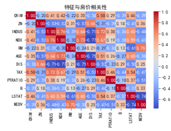

python 复制代码

# 将数据转换为均值为 0、标准差为 1的标准正态分布
from sklearn.preprocessing import StandardScaler
scaler = StandardScaler()
X_scaled = scaler.fit_transform(X)
from sklearn.linear_model import LinearRegression
from sklearn.model_selection import train_test_split
from sklearn.metrics import mean_squared_error, r2_score

# 划分训练集/测试集
X_train, X_test, y_train, y_test = train_test_split(X_scaled, y, test_size=0.2, random_state=42)

# 训练与评估
lr = LinearRegression()
lr.fit(X_train, y_train)
y_pred = lr.predict(X_test)

print(f"线性回归性能:")
print(f"RMSE: {np.sqrt(mean_squared_error(y_test, y_pred)):.2f}")#反映预测值与真实值的绝对偏差
print(f"R²: {r2_score(y_test, y_pred):.4f}") # 衡量模型拟合优度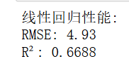

python 复制代码

from sklearn.ensemble import RandomForestRegressor
from sklearn.pipeline import Pipeline

# 构建流水线（标准化+模型）
pipeline = Pipeline([
    ('scaler', StandardScaler()),
    ('regressor', RandomForestRegressor(random_state=42))
])

# 训练与评估
pipeline.fit(X_train, y_train)
y_pred_rf = pipeline.predict(X_test)
print(f"随机森林初始性能:")
print(f"RMSE: {np.sqrt(mean_squared_error(y_test, y_pred_rf)):.2f}")
print(f"R²: {r2_score(y_test, y_pred_rf):.4f}")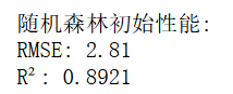

python 复制代码

plt.figure(figsize=(10, 6))
plt.scatter(y_test, y_pred, alpha=0.6, color='blue') 
plt.plot([y.min(), y.max()], [y.min(), y.max()], 'r--', lw=2)#X轴与Y轴范围
plt.xlabel('真实价格（千美元）')
plt.ylabel('预测价格（千美元）')
plt.title('真实值 vs 预测值')
plt.grid(True)
plt.show()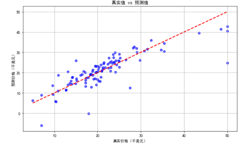

python 复制代码

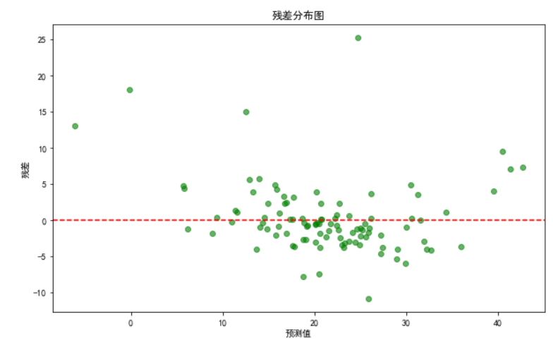
residuals = y_test - y_pred
plt.figure(figsize=(10, 6))
plt.scatter(y_pred, residuals, alpha=0.6, color='green')
plt.axhline(y=0, color='r', linestyle='--')
plt.xlabel('预测值')


plt.ylabel('残差')
plt.title('残差分布图')
plt.show()