R包fastWGCNA - 快速执行WGCNA分析和下游分析可视化

最新版本: 1.0.0
可以对着视频教程学习和使用：然而还没录呢, 关注B站等我更新

R包介绍

开发背景

WGCNA是转录组或芯片表达谱数据常用得分析, 可用来鉴定跟分组或表型相关得模块基因和核心基因
但其步骤非常之多, 每次运行起来很是费劲, 但需要修改的参数并不多
所以完全可以编写成一站式流程, 直接从表达谱和表型得到所有结果
另外得到模块基因后, 后续还有PPI和Cytoscape的分析

功能简介

一站式实现WGCNA, 只需要输入表达谱和分组或表型文件, 即可完成分析
保存各种结果文件, 如每个模块基因、hub基因、显著性结果、MM/GS评分等等
可视化内容: 散点图、相关性热图重绘、相关性蝴蝶图
下游分析: Cytoscape的MCODE和cytoHubba结果的提取和可视化

安装

没有安装包的需要付费获取安装包:
- 直接添加微信转账100, 发送fastR(依赖包)和fastWGCNA的压缩包
- 如果购买过R包fastGEO, 可以半价购买fastWGCNA包！
- 很多资料后面都会慢慢涨价, 早买会便宜很多!
- 购买后可进入交流群，后续版本更新和问题答疑都在群里进行
R包fastGEO目前售价调整为100, 以前为20, 逐步涨价到50, 现在是100
两包合购限时优惠150, 限时多久看心情
所有R包随着功能增加价格必然会上调, 早买早享受, 且免费获取最新版本

R 复制代码

# 依赖包
install_if_missing <- function(pkg, repos = getOption("repos")) {
    if (!requireNamespace(pkg, quietly = TRUE)) {
        install.packages(pkg, repos = repos)
    }
}

install_if_missing("WGCNA")
install_if_missing("linkET")
install_if_missing("dplyr")
install_if_missing("pdftools")
install_if_missing("UpSetR")
install_if_missing("VennDiagram")
install_if_missing("gridExtra")

R 复制代码

# 如果不存在fastR包或版本过低则进行安装
file_pkgs = grep("^fastR.*\\.gz$", dir(), value = TRUE)
if(!require("fastR", quietly = TRUE) || packageVersion("fastR") < strsplit(file_pkgs, "_|\\.tar")[[1]][2]){
    install.packages(file_pkgs, repos = NULL, upgrade = FALSE, force = TRUE)
}

R 复制代码

# 如果不存在fastWGCNA包或版本过低则进行安装
file_pkgs = grep("^fastWGCNA.*\\.gz$", dir(), value = TRUE)
if(!require("fastWGCNA", quietly = TRUE) || packageVersion("fastWGCNA") < strsplit(file_pkgs, "_|\\.tar")[[1]][2]){
    install.packages(file_pkgs, repos = NULL, upgrade = FALSE, force = TRUE)
}

R 复制代码

========================================
  欢迎使用 fastWGCNA (版本 1.0.0)
  - 作者: 生信摆渡
  - 微信: bioinfobaidu1
  - 帮助文档: help(package = fastWGCNA)
========================================

功能演示

R 复制代码

library(fastWGCNA)

R 复制代码

# 准备数据, 没有购买fastGEO的可以联系我购买或跳过此步
# 此步仅是数据准备, 也可以自行准备, 然后运行 run_WGCNA
library(fastGEO)

r 复制代码

========================================
  欢迎使用 fastGEO (版本 1.7.0)
  - 作者: 生信摆渡
  - 微信: bioinfobaidu1
  - 帮助文档: help(package = fastGEO)
========================================

run_WGCNA

一站式运行WGCNA, 需要输入表达谱(expM)和分组向量(group)或表型数据框(pheno)
其他重要参数
- dir: 输出文件夹
- case_name: 实验组的名称
- pheno_name: 表型的名称, 会在图中显示
- ntop: 选取方差最大的前多少基因构建网络, 越少运行速度越快。当模块数或结果基因较少时, 可以调多一点, 默认5000
- npower: 软阈值计算的最大值, 默认是20, 一般就够了, 样本太少时可能需要调到30才会满足构建网络的需求
- cut: 去除离群样本的聚类数的高度, 大于该高度的会被去除, 默认不去
- soft: 选择的软阈值, 默认使用推荐的软阈值, 也可手动指定
- zlim: 相关性热图的相关性范围, 当相关性不高时, 范围调窄点会更好看些
- minModuleSize: 每个模块最小的基因数, 默认30, 最低了
- deepSplit: 数值越大（通常0-4），模块划分越精细，会产生更多更小的模块, 默认2
- reassignThreshold: 基因重新分配的阈值, 影响模块的纯度，较高的阈值可能保留更多模糊归属的基因, 默认0
- mergeCutHeight: 基于模块间的相关性进行合并，值越大，合并的模块越多, 默认0.25
- corr_cutoff: 判定模块显著性的相关系数, 默认为0, 只要P值<0.05就行, 最低阈值
- pvalue_cutoff: 判定模块显著性的P值, 默认0.05
- MM_cutoff: MM阈值, 默认0.8
- GS_cutoff: GS阈值, 默认0.3
如果没有得到显著的模块, 可以调整以下参数:
- ntop调大, 最大为nrow(expM), 即所有基因
- deepSplit调大
- mergeCutHeight调小
如果没有得到hub基因或太少, 可以调整以下参数:
- MM调低，最小为0.3
- GS调低，最小为0.3

R 复制代码

obj = download_GEO("GSE30999", out_dir = "test/00_GEO_data_GSE30999")

r 复制代码

INFO [2025-08-27 11:17:17] Step1: Download GEO data ...
INFO [2025-08-27 11:17:17] Querying dataset: GSE30999 ...
	- Use local curl
	- Found 1 GPL
	- Found 170 samples, 39 metas.
	- Writting sample_anno to test/00_GEO_data_GSE30999/GSE30999_sample_anno.csv 
	- Normalize between arrays ...
	- Successed, file save to test/00_GEO_data_GSE30999/GSE30999_GPL570.RData.
INFO [2025-08-27 11:17:44] Step2: Annotate probe GPL570 ...
INFO [2025-08-27 11:17:45] Use built-in annotation file ...
- All porbes matched!
- All porbes annotated!
INFO [2025-08-27 11:17:46] Removing duplicated genes by method: max ...
INFO [2025-08-27 11:18:29] Done.

R 复制代码

gruop_list = get_GEO_group(obj, group_name = "source_name_ch1", "NL" = "Control", "LS" = "Psoriasis")
expM = gruop_list$expM
group = gruop_list$group

R 复制代码

hd(expM)

r 复制代码

Type: data.frame  Dim: 22881 × 170 
         GSM767976 GSM767978 GSM767980 GSM767982 GSM767984
A1BG      2.085353  2.079059  2.086824  2.081765  2.082029
A1BG-AS1  3.634412  2.953882  4.084853  3.958588  4.157088
A1CF      2.433706  2.395676  2.432235  2.381176  2.414382
A2M      13.489853 12.870176 12.957765 13.594529 13.878676
A2M-AS1   5.659882  4.673235  4.218735  5.400971  6.311412

R 复制代码

table(group)

r 复制代码

group
  Control Psoriasis 
       85        85

R 复制代码

# expM和group可自行准备
WGCNA_res = run_WGCNA(expM, group, case_name = "Psoriasis", pheno_name = "Psoriasis", dir = "test/GSE30999_WGCNA")

r 复制代码

Select top 5000 genes with largest variation ...

Check data integrity ...

	This a good data, nothing to do!

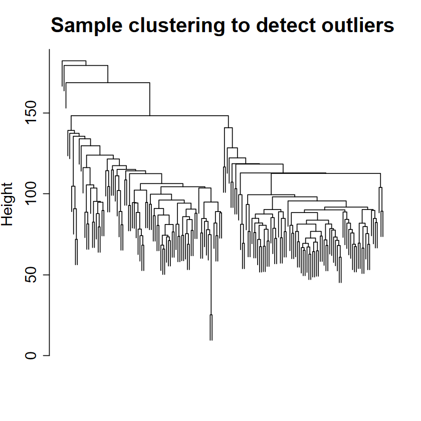
Detect outlier samples ...

Show_outlier samples

	Remove 0 sample(s)

Cluster with pheno

Determine soft threshold ...

Warning message:
"executing %dopar% sequentially: no parallel backend registered"
	Not specify soft threshold, using estimated: 6

	Scale independence

	Mean connectivity

Build modules ...

Plot Cluster dendrogram ...

Plot eigengene dendrogram ...

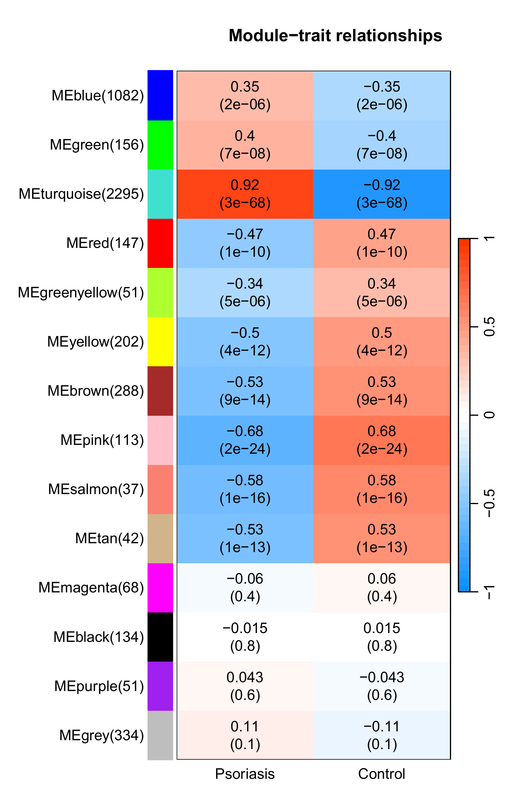
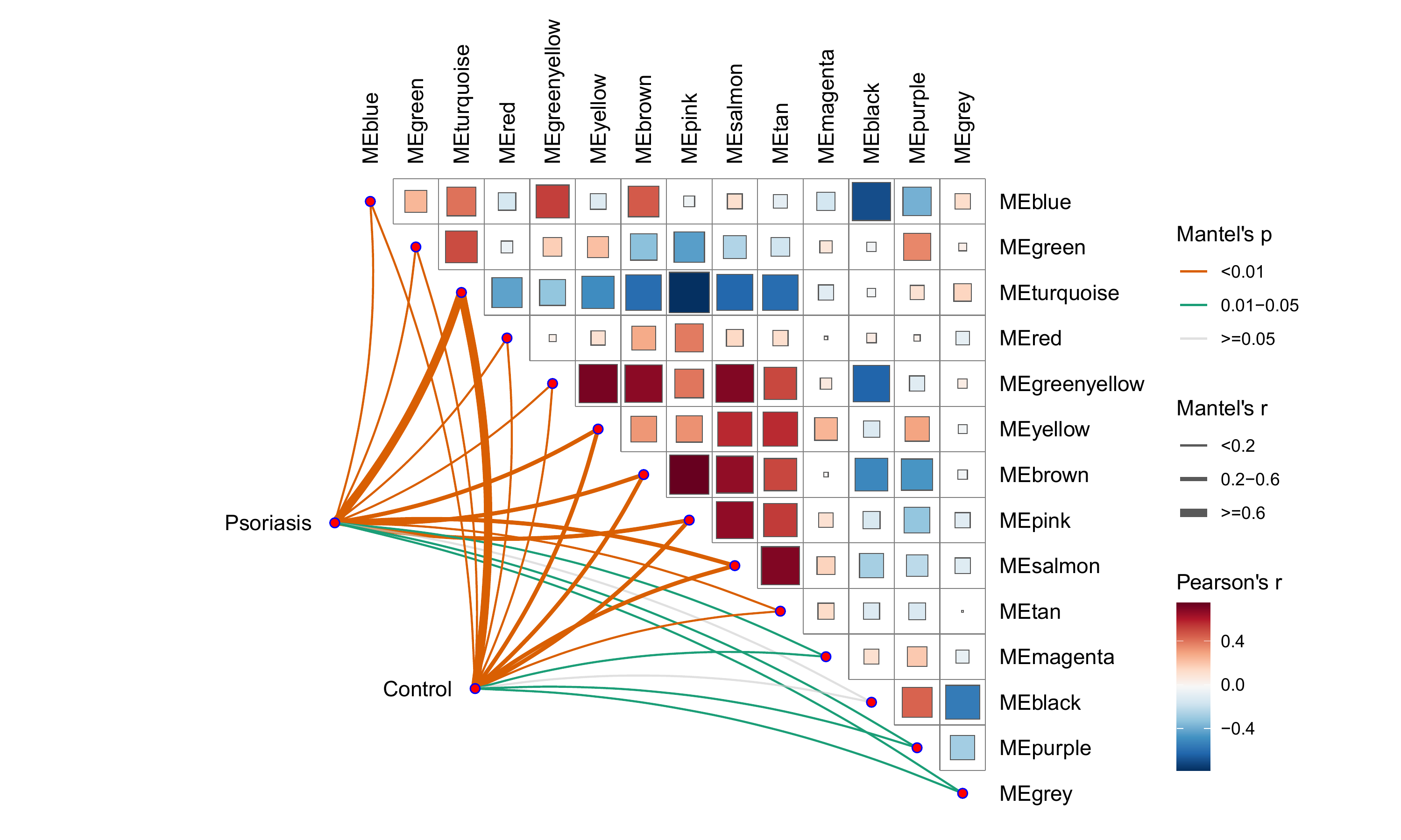
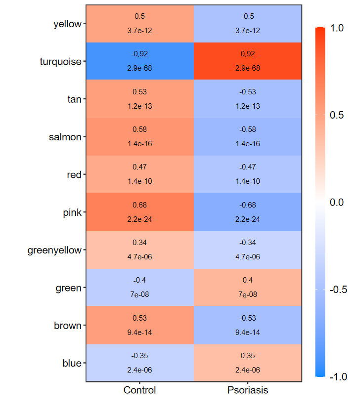
Show correlation and P-value between modules and phenos ...

Plot butterfly corrplot ...

Convert pdf to png ...

输出对象

R 复制代码

str(WGCNA_res)

r 复制代码

List of 12
 $ datExpr         : num [1:170, 1:5000] 2.27 8.36 2.68 2.62 9.24 ...
  ..- attr(*, "dimnames")=List of 2
  .. ..$ : chr [1:170] "GSM767976" "GSM767978" "GSM767980" "GSM767982" ...
  .. ..$ : chr [1:5000] "SERPINB4" "S100A12" "TCN1" "XIST" ...
 $ datTraits       :'data.frame':	170 obs. of  2 variables:
  ..$ Psoriasis: num [1:170] 0 0 0 0 0 0 0 0 0 0 ...
  ..$ Control  : num [1:170] 1 1 1 1 1 1 1 1 1 1 ...
 $ MEs             :'data.frame':	170 obs. of  14 variables:
  ..$ MEblue       : num [1:170] -0.0477 -0.169 -0.1571 -0.1265 -0.0532 ...
  ..$ MEgreen      : num [1:170] 0.0133 0.0231 -0.0146 -0.1468 -0.2191 ...
  ..$ MEturquoise  : num [1:170] -0.0726 -0.0644 -0.0859 -0.1298 -0.0848 ...
  ..$ MEred        : num [1:170] 0.0146 -0.0218 0.1047 0.0307 -0.0513 ...
  ..$ MEgreenyellow: num [1:170] 0.08038 -0.00806 -0.00954 -0.03715 -0.00169 ...
  ..$ MEyellow     : num [1:170] 0.0887 0.1067 0.0628 0.0196 -0.0385 ...
  ..$ MEbrown      : num [1:170] -0.00425 -0.06434 -0.064 0.04502 0.04749 ...
  ..$ MEpink       : num [1:170] -0.0199 -0.0351 0.0287 0.1011 0.1063 ...
  ..$ MEsalmon     : num [1:170] 0.0711 -0.0173 0.0537 0.02 0.0896 ...
  ..$ MEtan        : num [1:170] 0.1622 0.0444 0.0503 0.1119 0.1766 ...
  ..$ MEmagenta    : num [1:170] 0.0472 0.037 0.0825 -0.0614 -0.0482 ...
  ..$ MEblack      : num [1:170] -0.07746 0.04469 -0.01769 -0.00823 -0.03659 ...
  ..$ MEpurple     : num [1:170] 0.0446 0.0721 -0.0119 -0.0994 -0.1468 ...
  ..$ MEgrey       : num [1:170] 0.1167 0.0228 0.076 0.1295 0.0814 ...
 $ all_module_genes:List of 14
  ..$ blue       : chr [1:1082] "ABCB1" "ABCC10" "ABHD14A-ACY1" "ABHD2" ...
  ..$ green      : chr [1:156] "AIF1" "ALOX5AP" "AMICA1" "B3GNT7" ...
  ..$ turquoise  : chr [1:2295] "A2ML1" "A2MP1" "AAMDC" "AASS" ...
  ..$ red        : chr [1:147] "ABCA13" "ACAA2" "ACADM" "ACAT2" ...
  ..$ greenyellow: chr [1:51] "ACAD8" "AF007147" "AFAP1L1" "AMIGO2" ...
  ..$ yellow     : chr [1:202] "ABCA6" "ABI3BP" "ACKR4" "ACVRL1" ...
  ..$ brown      : chr [1:288] "ABAT" "ACCS" "ACTG1P4" "ADCY10P1" ...
  ..$ pink       : chr [1:113] "AACSP1" "AB488780" "ABO" "ACACB" ...
  ..$ salmon     : chr [1:37] "ABLIM3" "ACTA1" "ACTC1" "ACTG2" ...
  ..$ tan        : chr [1:42] "ACVR1C" "ADIPOQ" "AIFM2" "AQP7" ...
  ..$ magenta    : chr [1:68] "ANGPTL7" "CAPN8" "CBLN2" "COL11A1" ...
  ..$ black      : chr [1:134] "ADAT1" "AK091729" "ALOX5" "AP006216.10" ...
  ..$ purple     : chr [1:51] "AADAC" "ACER1" "AF086294" "ASPHD2" ...
  ..$ grey       : chr [1:334] "ABCC4" "abParts" "ABTB2" "AC007362.3" ...
 $ signif_summary  :List of 2
  ..$ Psoriasis:'data.frame':	14 obs. of  4 variables:
  .. ..$ corr  : num [1:14] 0.353 0.399 0.915 -0.467 -0.343 ...
  .. ..$ pvalue: num [1:14] 2.40e-06 6.96e-08 2.87e-68 1.35e-10 4.68e-06 ...
  .. ..$ Ngene : int [1:14] 1082 156 2295 147 51 202 288 113 37 42 ...
  .. ..$ Sig   : chr [1:14] "POS" "POS" "POS" "NEG" ...
  ..$ Control  :'data.frame':	14 obs. of  4 variables:
  .. ..$ corr  : num [1:14] -0.353 -0.399 -0.915 0.467 0.343 ...
  .. ..$ pvalue: num [1:14] 2.40e-06 6.96e-08 2.87e-68 1.35e-10 4.68e-06 ...
  .. ..$ Ngene : int [1:14] 1082 156 2295 147 51 202 288 113 37 42 ...
  .. ..$ Sig   : chr [1:14] "NEG" "NEG" "NEG" "POS" ...
 $ moduleLabels    : Named num [1:5000] 1 1 1 0 0 6 1 1 0 1 ...
  ..- attr(*, "names")= chr [1:5000] "SERPINB4" "S100A12" "TCN1" "XIST" ...
 $ moduleColors    : chr [1:5000] "turquoise" "turquoise" "turquoise" "grey" ...
 $ geneTree        :List of 7
  ..$ merge      : int [1:4999, 1:2] -15 -40 -39 -71 -63 -4 -5 -89 -459 -106 ...
  ..$ height     : num [1:4999] 0.146 0.152 0.153 0.158 0.166 ...
  ..$ order      : int [1:5000] 4355 9 128 2563 4125 712 4990 1436 1489 2812 ...
  ..$ labels     : NULL
  ..$ method     : chr "average"
  ..$ call       : language fastcluster::hclust(d = as.dist(dissTom), method = "average")
  ..$ dist.method: NULL
  ..- attr(*, "class")= chr "hclust"
 $ all_module_genes:List of 14
  ..$ blue       : chr [1:1082] "ABCB1" "ABCC10" "ABHD14A-ACY1" "ABHD2" ...
  ..$ green      : chr [1:156] "AIF1" "ALOX5AP" "AMICA1" "B3GNT7" ...
  ..$ turquoise  : chr [1:2295] "A2ML1" "A2MP1" "AAMDC" "AASS" ...
  ..$ red        : chr [1:147] "ABCA13" "ACAA2" "ACADM" "ACAT2" ...
  ..$ greenyellow: chr [1:51] "ACAD8" "AF007147" "AFAP1L1" "AMIGO2" ...
  ..$ yellow     : chr [1:202] "ABCA6" "ABI3BP" "ACKR4" "ACVRL1" ...
  ..$ brown      : chr [1:288] "ABAT" "ACCS" "ACTG1P4" "ADCY10P1" ...
  ..$ pink       : chr [1:113] "AACSP1" "AB488780" "ABO" "ACACB" ...
  ..$ salmon     : chr [1:37] "ABLIM3" "ACTA1" "ACTC1" "ACTG2" ...
  ..$ tan        : chr [1:42] "ACVR1C" "ADIPOQ" "AIFM2" "AQP7" ...
  ..$ magenta    : chr [1:68] "ANGPTL7" "CAPN8" "CBLN2" "COL11A1" ...
  ..$ black      : chr [1:134] "ADAT1" "AK091729" "ALOX5" "AP006216.10" ...
  ..$ purple     : chr [1:51] "AADAC" "ACER1" "AF086294" "ASPHD2" ...
  ..$ grey       : chr [1:334] "ABCC4" "abParts" "ABTB2" "AC007362.3" ...
 $ signif_summary  :List of 2
  ..$ Psoriasis:'data.frame':	14 obs. of  4 variables:
  .. ..$ corr  : num [1:14] 0.353 0.399 0.915 -0.467 -0.343 ...
  .. ..$ pvalue: num [1:14] 2.40e-06 6.96e-08 2.87e-68 1.35e-10 4.68e-06 ...
  .. ..$ Ngene : int [1:14] 1082 156 2295 147 51 202 288 113 37 42 ...
  .. ..$ Sig   : chr [1:14] "POS" "POS" "POS" "NEG" ...
  ..$ Control  :'data.frame':	14 obs. of  4 variables:
  .. ..$ corr  : num [1:14] -0.353 -0.399 -0.915 0.467 0.343 ...
  .. ..$ pvalue: num [1:14] 2.40e-06 6.96e-08 2.87e-68 1.35e-10 4.68e-06 ...
  .. ..$ Ngene : int [1:14] 1082 156 2295 147 51 202 288 113 37 42 ...
  .. ..$ Sig   : chr [1:14] "NEG" "NEG" "NEG" "POS" ...
 $ sinif_genes     :List of 2
  ..$ Psoriasis: chr [1:4413] "A2ML1" "A2MP1" "AACSP1" "AAMDC" ...
  ..$ Control  : chr [1:4413] "A2ML1" "A2MP1" "AACSP1" "AAMDC" ...
 $ hub_genes       :List of 14
  ..$ blue       :'data.frame':	0 obs. of  2 variables:
  .. ..$ MM: num(0) 
  .. ..$ GS: num(0) 
  ..$ green      :'data.frame':	0 obs. of  2 variables:
  .. ..$ MM: num(0) 
  .. ..$ GS: num(0) 
  ..$ turquoise  :'data.frame':	174 obs. of  2 variables:
  .. ..$ MM: num [1:174] 0.95 0.969 0.943 0.956 0.957 ...
  .. ..$ GS: num [1:174] 0.923 0.953 0.928 0.912 0.936 ...
  ..$ red        :'data.frame':	0 obs. of  2 variables:
  .. ..$ MM: num(0) 
  .. ..$ GS: num(0) 
  ..$ greenyellow:'data.frame':	0 obs. of  2 variables:
  .. ..$ MM: num(0) 
  .. ..$ GS: num(0) 
  ..$ yellow     :'data.frame':	0 obs. of  2 variables:
  .. ..$ MM: num(0) 
  .. ..$ GS: num(0) 
  ..$ brown      :'data.frame':	0 obs. of  2 variables:
  .. ..$ MM: num(0) 
  .. ..$ GS: num(0) 
  ..$ pink       :'data.frame':	2 obs. of  2 variables:
  .. ..$ MM: num [1:2] 0.863 0.865
  .. ..$ GS: num [1:2] 0.803 0.82
  ..$ salmon     :'data.frame':	0 obs. of  2 variables:
  .. ..$ MM: num(0) 
  .. ..$ GS: num(0) 
  ..$ tan        :'data.frame':	0 obs. of  2 variables:
  .. ..$ MM: num(0) 
  .. ..$ GS: num(0) 
  ..$ magenta    :'data.frame':	0 obs. of  2 variables:
  .. ..$ MM: num(0) 
  .. ..$ GS: num(0) 
  ..$ black      :'data.frame':	0 obs. of  2 variables:
  .. ..$ MM: num(0) 
  .. ..$ GS: num(0) 
  ..$ purple     :'data.frame':	0 obs. of  2 variables:
  .. ..$ MM: num(0) 
  .. ..$ GS: num(0) 
  ..$ grey       :'data.frame':	0 obs. of  2 variables:
  .. ..$ MM: num(0) 
  .. ..$ GS: num(0)

输出目录
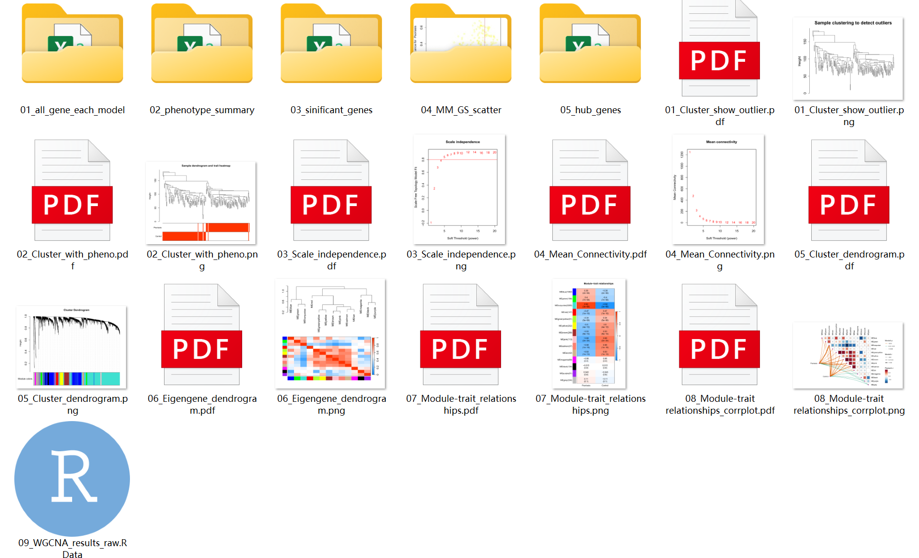
01_all_gene_each_model: 每个模块的所有基因
02_phenotype_summary: 显著性统计表, 可用作后续筛选
03_sinificant_genes: 对应相关系数和p值下所有显著模块的基因
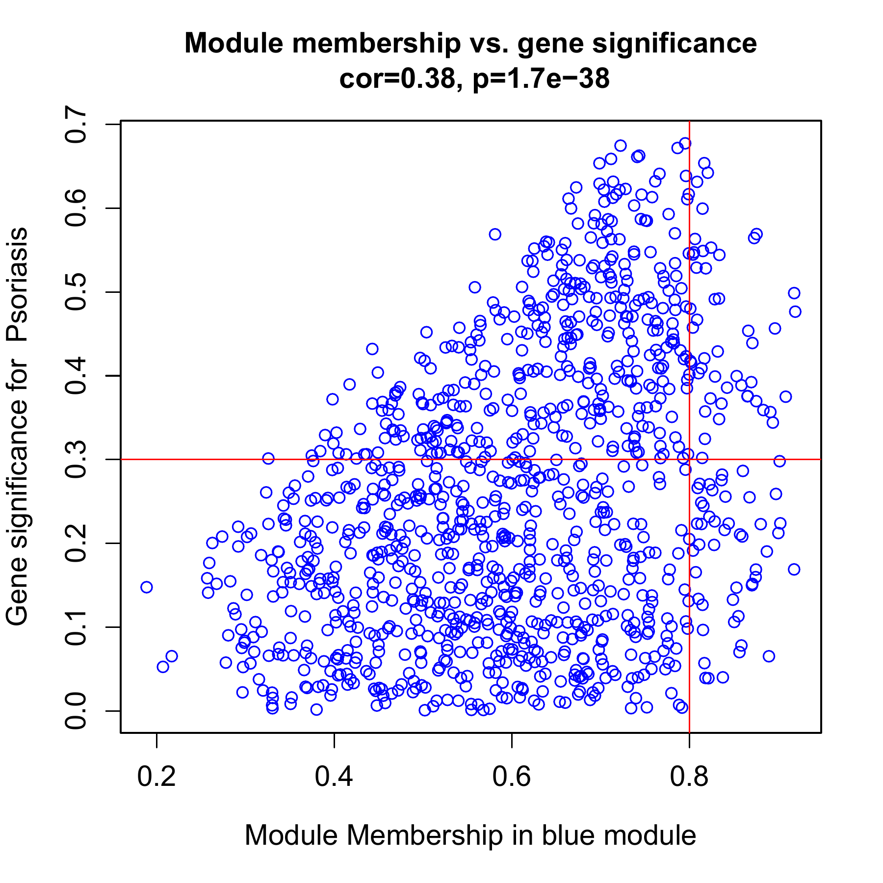
04_MM_GS_scatter: 每个模块
前面常规的图就不多解释了, 全都是发表级别的图
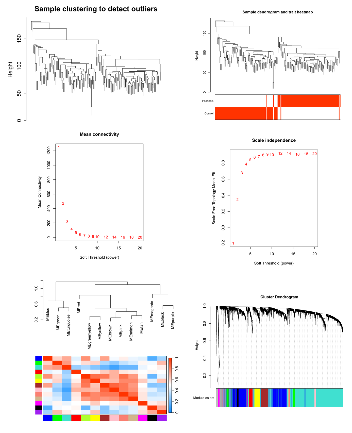
相关性热图增加了每个模块的基因数
这很重要不是吗? 是我们决定选择哪个模块或判断结果可不可用的关键因素。
相关性蝴蝶图
相关性的另外一种展示, 还怪好看的
MM MS相关性图
如果进行了hub筛选, 这个图是必须要放的, 每个模块一个图

extractMCODE

对Cytoscape MCODE插件输出结果进行提取和分析
输出原始表格、每一子网络的基因集及其GO富集分析结果

R 复制代码

extractMCODE("./test/PPI_MCODE.txt", runGO = FALSE)

R 复制代码

$clusterT
A data.frame: 3 × 5
Cluster	Score	Nodes	Edges	IDs
<int>	<dbl>	<int>	<int>	<chr>
1	5.429	8	19	CDK2, PDGFB, VEGFC, CCND2, NOTCH1, KIT, CCND1, EPHA2
2	3.000	3	3	PKP2, KCNH2, TMEM43
3	3.000	3	3	HBA1, HBB, HBA2
$cluster_list
$Cluster1
	'CDK2''PDGFB''VEGFC''CCND2''NOTCH1''KIT''CCND1''EPHA2'
$Cluster2
	'PKP2''KCNH2''TMEM43'
$Cluster3
	'HBA1''HBB''HBA2'

R 复制代码

# 对每一CLuster富集分析, 耗时
mcode_res = extractMCODE("./test/PPI_MCODE.txt")

r 复制代码

Loading packages ...

Running ONTOLOGY: ALL ...

782  terms enriched

Loading packages ...

Running ONTOLOGY: ALL ...

143  terms enriched

Loading packages ...

Running ONTOLOGY: ALL ...

55  terms enriched

R 复制代码

str(mcode_res$egoL)

r 复制代码

List of 3
 $ Cluster1:'data.frame':	782 obs. of  10 variables:
  ..$ ONTOLOGY   : chr [1:782] "BP" "BP" "BP" "BP" ...
  ..$ ID         : chr [1:782] "GO:1904238" "GO:0033674" "GO:0060326" "GO:0071902" ...
  ..$ Description: chr [1:782] "pericyte cell differentiation" "positive regulation of kinase activity" "cell chemotaxis" "positive regulation of protein serine/threonine kinase activity" ...
  ..$ GeneRatio  : chr [1:782] "3/8" "5/8" "5/8" "4/8" ...
  ..$ BgRatio    : chr [1:782] "11/21288" "346/21288" "375/21288" "140/21288" ...
  ..$ pvalue     : num [1:782] 5.74e-09 5.93e-08 8.86e-08 1.23e-07 1.27e-07 ...
  ..$ p.adjust   : num [1:782] 5.74e-06 2.00e-05 2.00e-05 2.00e-05 2.00e-05 ...
  ..$ qvalue     : num [1:782] 1.62e-06 5.63e-06 5.63e-06 5.63e-06 5.63e-06 ...
  ..$ geneID     : chr [1:782] "PDGFB/NOTCH1/EPHA2" "PDGFB/CCND2/KIT/CCND1/EPHA2" "PDGFB/VEGFC/NOTCH1/KIT/EPHA2" "PDGFB/CCND2/KIT/CCND1" ...
  ..$ Count      : int [1:782] 3 5 5 4 5 5 5 5 4 3 ...
 $ Cluster2:'data.frame':	143 obs. of  10 variables:
  ..$ ONTOLOGY   : chr [1:143] "BP" "BP" "BP" "BP" ...
  ..$ ID         : chr [1:143] "GO:0086005" "GO:0086091" "GO:0086002" "GO:0086003" ...
  ..$ Description: chr [1:143] "ventricular cardiac muscle cell action potential" "regulation of heart rate by cardiac conduction" "cardiac muscle cell action potential involved in contraction" "cardiac muscle cell contraction" ...
  ..$ GeneRatio  : chr [1:143] "2/3" "2/3" "2/3" "2/3" ...
  ..$ BgRatio    : chr [1:143] "37/21288" "44/21288" "63/21288" "86/21288" ...
  ..$ pvalue     : num [1:143] 8.81e-06 1.25e-05 2.58e-05 4.83e-05 4.94e-05 ...
  ..$ p.adjust   : num [1:143] 0.000669 0.000669 0.000921 0.001057 0.001057 ...
  ..$ qvalue     : num [1:143] 4.61e-05 4.61e-05 6.34e-05 7.28e-05 7.28e-05 ...
  ..$ geneID     : chr [1:143] "PKP2/KCNH2" "PKP2/KCNH2" "PKP2/KCNH2" "PKP2/KCNH2" ...
  ..$ Count      : int [1:143] 2 2 2 2 2 2 2 2 2 2 ...
 $ Cluster3:'data.frame':	55 obs. of  10 variables:
  ..$ ONTOLOGY   : chr [1:55] "BP" "BP" "BP" "BP" ...
  ..$ ID         : chr [1:55] "GO:0015670" "GO:0015671" "GO:0015669" "GO:0019755" ...
  ..$ Description: chr [1:55] "carbon dioxide transport" "oxygen transport" "gas transport" "one-carbon compound transport" ...
  ..$ GeneRatio  : chr [1:55] "3/3" "3/3" "3/3" "3/3" ...
  ..$ BgRatio    : chr [1:55] "15/21288" "15/21288" "22/21288" "26/21288" ...
  ..$ pvalue     : num [1:55] 2.83e-10 2.83e-10 9.58e-10 1.62e-09 2.80e-09 ...
  ..$ p.adjust   : num [1:55] 5.24e-09 5.24e-09 1.18e-08 1.50e-08 2.07e-08 ...
  ..$ qvalue     : num [1:55] 2.98e-10 2.98e-10 6.72e-10 8.51e-10 1.18e-09 ...
  ..$ geneID     : chr [1:55] "HBA1/HBB/HBA2" "HBA1/HBB/HBA2" "HBA1/HBB/HBA2" "HBA1/HBB/HBA2" ...
  ..$ Count      : int [1:55] 3 3 3 3 3 3 3 3 3 3 ...

R 复制代码

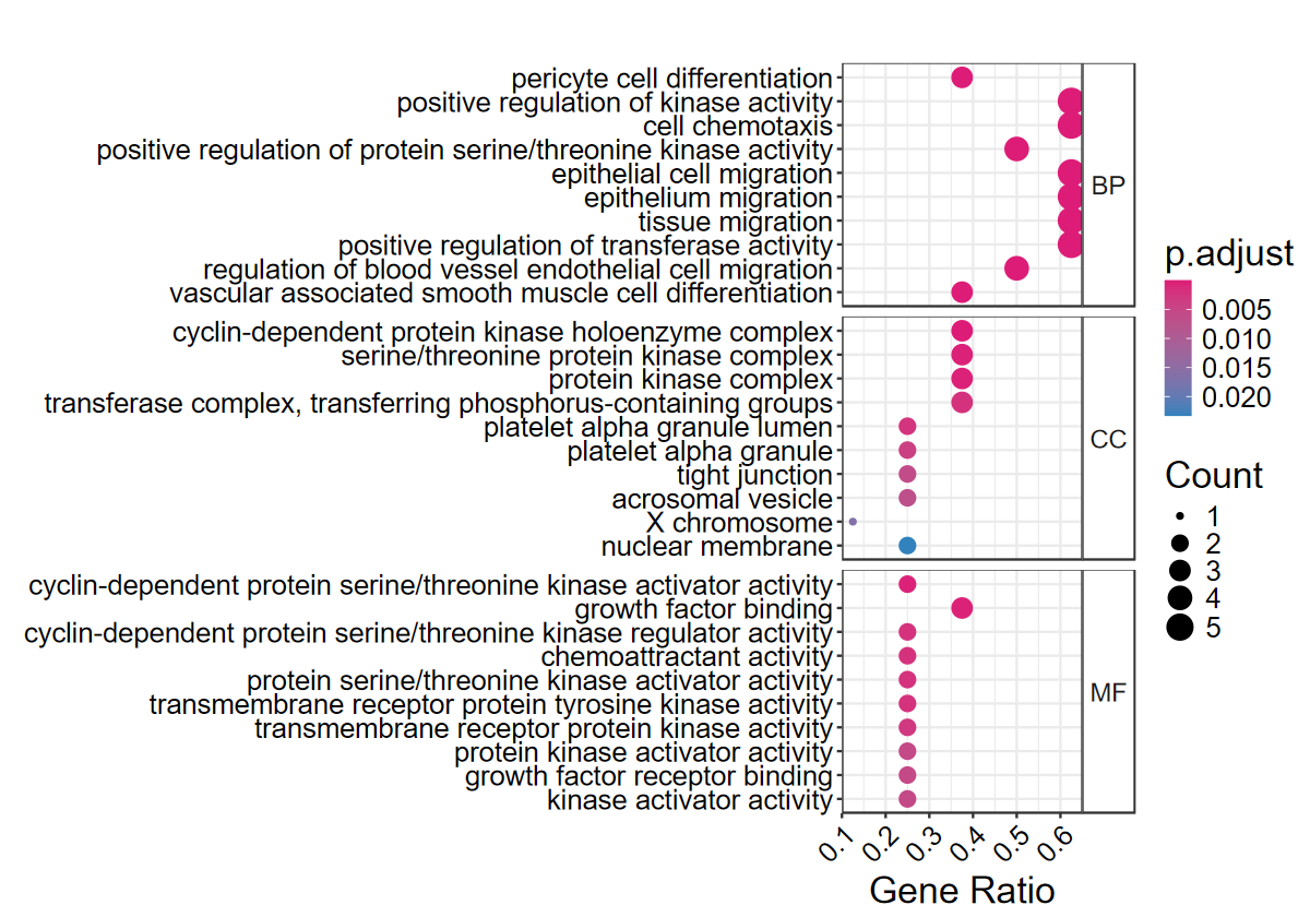
# 简单看下气泡图
set_image(10, 7)
dotplotGO(mcode_res$egoL$Cluster1)

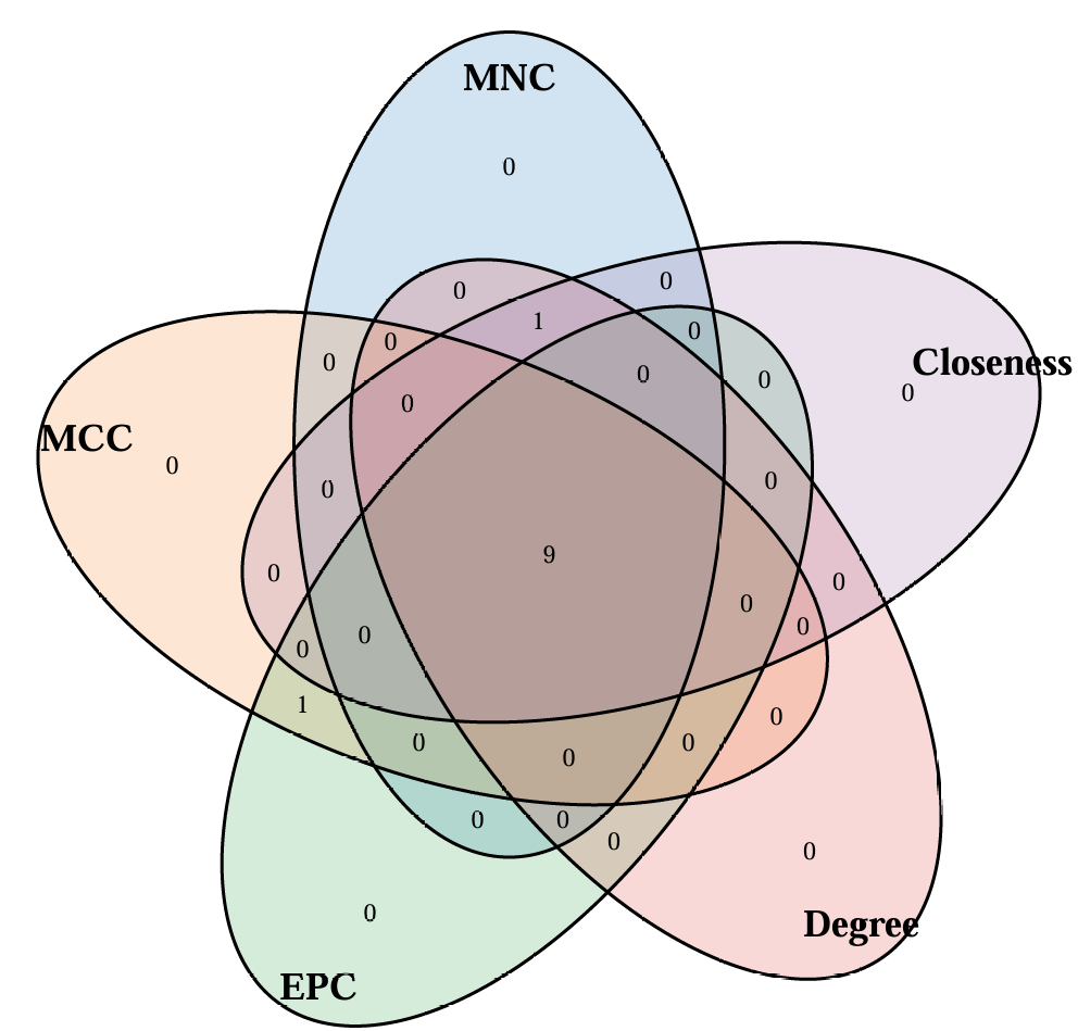
plot_cytohubba_intersection

对Cytoscape cytoHubb 插件输出结果进行提取和分析
提取常用的5种算法的 top N 个基因取交集, 并绘制韦恩图和upset图

R 复制代码

cytohubba_res = plot_cytohubba_intersection("./test/PPI_CytoHubba.csv", out_name = "./test/PPI_CytoHubba")

R 复制代码

cytohubba_res

r 复制代码

$top_genes
$top_genes$MNC
 [1] "XDH"     "IL1B"    "HMOX1"   "PLAT"    "PPARG"   "HMOX2"   "PRKCB"  
 [8] "BLVRA"   "POR"     "SULT1A3"

$top_genes$MCC
 [1] "XDH"   "IL1B"  "HMOX1" "PPARG" "PLAT"  "HMOX2" "BLVRA" "PRKCB" "POR"  
[10] "PTGES"

$top_genes$EPC
 [1] "XDH"   "IL1B"  "HMOX1" "PPARG" "PLAT"  "HMOX2" "PRKCB" "BLVRA" "POR"  
[10] "PTGES"

$top_genes$Degree
 [1] "XDH"     "IL1B"    "HMOX1"   "PLAT"    "PPARG"   "HMOX2"   "PRKCB"  
 [8] "BLVRA"   "POR"     "SULT1A3"

$top_genes$Closeness
 [1] "XDH"     "IL1B"    "HMOX1"   "PLAT"    "PPARG"   "HMOX2"   "PRKCB"  
 [8] "BLVRA"   "POR"     "SULT1A3"


$common_genes
[1] "BLVRA" "HMOX1" "HMOX2" "IL1B"  "PLAT"  "POR"   "PPARG" "PRKCB" "XDH"  

$files_generated
[1] "./test/PPI_CytoHubba_upset.pdf"       
[2] "./test/PPI_CytoHubba_venn.pdf"        
[3] "./test/PPI_CytoHubba_common_genes.csv"

upset图：
韦恩图：

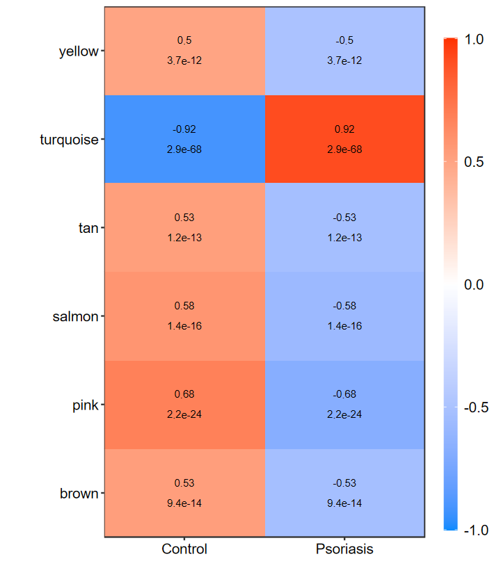
heatmap_replot

重新绘制相关性热图, 用于当模块数过多时
不大好看, 几年前写的了, 后面再优化
已发表的论文用过我做的这个图了, 关键信息都有了

R 复制代码

# 只显示显著的
set_image(6, 7)
heatmap_replot(WGCNA_res$signif_summary)

R 复制代码

# 自定义显示的阈值
heatmap_replot(WGCNA_res$signif_summary, pvalue = 0.001, corr = 0.5)

get_hub_genes

待开发
根据相关性阈值和MM/GS阈值重新提取hub基因
目前根据返回的 WGCNA_res 对象有点R基础的也能自行提取