用LightGBM解决多元回归与时间序列问题：5折交叉验证与Hyperopt超参数优化实战

LightGBM用于多元回归或者时间序列问题。包括5折交叉验证和hyperopt超参数优化自带数据集可以直接运行，有结果曲线图和评价指标 python 程序

在数据科学领域，LightGBM 以其高效性和准确性备受青睐。今天，咱们就来聊聊如何运用 LightGBM 处理多元回归或者时间序列问题，同时结合 5 折交叉验证与 Hyperopt 超参数优化，还会展示如何使用自带数据集直接运行，最后生成结果曲线图并给出评价指标。

多元回归示例

数据准备

咱们先用 sklearn 自带的波士顿房价数据集作为多元回归的示例数据。这个数据集有多个特征，目标是预测房价。

python 复制代码

from sklearn.datasets import load_boston
from sklearn.model_selection import train_test_split
import lightgbm as lgb
import numpy as np
import pandas as pd
from hyperopt import hp, fmin, tpe, STATUS_OK
from sklearn.model_selection import cross_val_score
import matplotlib.pyplot as plt
from sklearn.metrics import mean_squared_error, r2_score

# 加载波士顿房价数据集
boston = load_boston()
X = pd.DataFrame(boston.data, columns=boston.feature_names)
y = boston.target

# 划分训练集和测试集
X_train, X_test, y_train, y_test = train_test_split(X, y, test_size=0.2, random_state=42)

在这段代码里，首先从 sklearn.datasets 导入 loadboston**来加载数据集，接着用 pandas 将特征数据转换为 DataFrame 方便后续操作，然后使用 train testsplit**把数据按 80%训练集、20%测试集划分，random state 设置为固定值以保证每次运行结果一致。

5 折交叉验证

在训练模型之前，咱们先进行 5 折交叉验证来评估模型的稳定性。

python 复制代码

# 定义LightGBM模型
lgb_model = lgb.LGBMRegressor()

# 5折交叉验证
cv_scores = cross_val_score(lgb_model, X_train, y_train, cv=5, scoring='neg_mean_squared_error')
print("5折交叉验证的MSE得分：", -cv_scores)

这里先初始化一个 LGBMRegressor 模型，然后调用 crossvalscore 函数，设置 cv=5 进行 5 折交叉验证，scoring='negmeansquared_error' 表示使用负均方误差作为评估指标，最后打印出每次交叉验证的得分。

Hyperopt 超参数优化

接下来，用 Hyperopt 对模型超参数进行优化。

python 复制代码

# 定义超参数搜索空间
space = {
    'n_estimators': hp.quniform('n_estimators', 100, 1000, 10),
    'learning_rate': hp.loguniform('learning_rate', np.log(0.01), np.log(0.3)),
   'max_depth': hp.quniform('max_depth', 3, 10, 1),
    'num_leaves': hp.quniform('num_leaves', 20, 100, 5)
}


# 定义目标函数
def objective(params):
    model = lgb.LGBMRegressor(
        n_estimators=int(params['n_estimators']),
        learning_rate=params['learning_rate'],
        max_depth=int(params['max_depth']),
        num_leaves=int(params['num_leaves'])
    )
    cv_scores = cross_val_score(model, X_train, y_train, cv=5, scoring='neg_mean_squared_error')
    return {'loss': -np.mean(cv_scores),'status': STATUS_OK}


# 超参数优化
best = fmin(fn=objective, space=space, algo=tpe.suggest, max_evals=50)
print("最优超参数：", best)

在超参数搜索空间 space 里，咱们定义了 nestimators*（估计器数量）、learning* rate（学习率）、maxdepth*（最大深度）和 num* leaves（叶子节点数）的搜索范围。objective 函数接收超参数，初始化模型并进行 5 折交叉验证，返回平均负均方误差作为损失值。最后，fmin 函数通过 tpe.suggest 算法在搜索空间里进行 50 次评估找到最优超参数。

模型训练与评估

有了最优超参数，咱们就可以训练模型并评估了。

python 复制代码

# 使用最优超参数训练模型
best_model = lgb.LGBMRegressor(
    n_estimators=int(best['n_estimators']),
    learning_rate=best['learning_rate'],
    max_depth=int(best['max_depth']),
    num_leaves=int(best['num_leaves'])
)
best_model.fit(X_train, y_train)

# 模型预测
y_pred = best_model.predict(X_test)

# 计算评价指标
mse = mean_squared_error(y_test, y_pred)
r2 = r2_score(y_test, y_pred)
print("均方误差MSE：", mse)
print("R2得分：", r2)

这段代码使用最优超参数初始化模型并在训练集上训练，然后在测试集上预测。最后，用 meansquarederror 和 r2_score 计算均方误差和 R2 得分来评估模型性能。

结果曲线图绘制

为了更直观地看出预测效果，咱们绘制预测值和真实值的对比图。

python 复制代码

plt.scatter(y_test, y_pred)
plt.xlabel('真实值')
plt.ylabel('预测值')
plt.title('LightGBM多元回归预测结果')
plt.show()

这几行代码简单地用 matplotlib 绘制了散点图，横轴是真实值，纵轴是预测值，能直观地展示预测值和真实值的分布情况。

时间序列示例（以简单随机游走生成数据模拟）

数据生成

python 复制代码

# 生成简单随机游走时间序列数据
np.random.seed(42)
n = 100
time_series = np.cumsum(np.random.randn(n))
time = np.arange(n)

# 划分训练集和测试集
train_size = int(len(time_series) * 0.8)
X_train_time = time[:train_size].reshape(-1, 1)
y_train_time = time_series[:train_size]
X_test_time = time[train_size:].reshape(-1, 1)
y_test_time = time_series[train_size:]

这里用 numpy 生成了简单的随机游走时间序列数据，然后按 80%训练集、20%测试集划分。

同样的流程应用到时间序列

从 5 折交叉验证到超参数优化，再到模型训练评估和绘图，过程和多元回归类似，只不过这里数据是时间序列格式。

python 复制代码

# 定义LightGBM模型
lgb_model_time = lgb.LGBMRegressor()

# 5折交叉验证
cv_scores_time = cross_val_score(lgb_model_time, X_train_time, y_train_time, cv=5, scoring='neg_mean_squared_error')
print("时间序列5折交叉验证的MSE得分：", -cv_scores_time)

# 超参数搜索空间
space_time = {
    'n_estimators': hp.quniform('n_estimators', 100, 1000, 10),
    'learning_rate': hp.loguniform('learning_rate', np.log(0.01), np.log(0.3)),
   'max_depth': hp.quniform('max_depth', 3, 10, 1),
    'num_leaves': hp.quniform('num_leaves', 20, 100, 5)
}


# 目标函数
def objective_time(params):
    model = lgb.LGBMRegressor(
        n_estimators=int(params['n_estimators']),
        learning_rate=params['learning_rate'],
        max_depth=int(params['max_depth']),
        num_leaves=int(params['num_leaves'])
    )
    cv_scores = cross_val_score(model, X_train_time, y_train_time, cv=5, scoring='neg_mean_squared_error')
    return {'loss': -np.mean(cv_scores),'status': STATUS_OK}


# 超参数优化
best_time = fmin(fn=objective_time, space=space_time, algo=tpe.suggest, max_evals=50)
print("时间序列最优超参数：", best_time)

# 使用最优超参数训练模型
best_model_time = lgb.LGBMRegressor(
    n_estimators=int(best_time['n_estimators']),
    learning_rate=best_time['learning_rate'],
    max_depth=int(best_time['max_depth']),
    num_leaves=int(best_time['num_leaves'])
)
best_model_time.fit(X_train_time, y_train_time)

# 模型预测
y_pred_time = best_model_time.predict(X_test_time)

# 计算评价指标
mse_time = mean_squared_error(y_test_time, y_pred_time)
r2_time = r2_score(y_test_time, y_pred_time)
print("时间序列均方误差MSE：", mse_time)
print("时间序列R2得分：", r2_time)

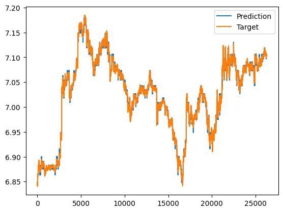
# 结果曲线图绘制
plt.plot(time[train_size:], y_test_time, label='真实值')
plt.plot(time[train_size:], y_pred_time, label='预测值')
plt.xlabel('时间')
plt.ylabel('值')
plt.title('LightGBM时间序列预测结果')
plt.legend()
plt.show()

通过上述步骤，无论是多元回归还是时间序列问题，我们都利用 LightGBM 结合 5 折交叉验证与 Hyperopt 超参数优化，实现了数据处理、模型训练评估以及可视化展示。这样的流程可以帮助我们更好地理解和运用 LightGBM 模型解决实际问题。

希望这篇博文能对你在处理多元回归或时间序列问题时有所帮助，赶紧动手试试吧！