CornerNet模型的复现

主题：仅仅用于个人论文复现的思考，如有不对，敬请指正

起因：之所以复现了ECCV2018年的论文是由于他的思想非常简洁，将目标检测问题转换为角点检测问题。启迪了Anchor---free检测思想。

传统依赖于anchor box的方法需要在图像上放置无数的anchor box以尽可能的保证与真实框的重叠。最终，只有一小部分和ground truth重叠，并且产生了严重的样本不均衡问题。

项目构建

神经网络搭建一般有一个默认的目录结构。当然，这个没有唯一，一般是取决于自己的范式。

目录架构

复制代码

CornerNet-Reproduction/
├── models/
│   ├── __init__.py
│   ├── backbone.py          # Hourglass网络
│   ├── corner_pool.py       # Corner Pooling实现
│   ├── cornernet.py         # 主网络
│   └── loss.py              # 损失函数
├── utils/
│   ├── __init__.py
│   ├── image.py             # 图像处理
│   ├── decode.py            # 推理解码
│   └── visualization.py     # 可视化工具
├── data/
│   ├── __init__.py
│   ├── coco.py              # COCO数据集
│   └── transforms.py        # 数据增强
├── configs/
│   └── cornernet_config.py  # 配置文件
├── train.py                 # 训练脚本
├── test.py                  # 测试脚本
├── demo.py                  # 演示脚本
└── requirements.txt         # 依赖包

equirements.txt

一般来说，所需要的python包俊在此处。这也是标准的范式。基本上所有的网络架构里面均是如此。

复制代码

# pip install -r requirements.txt
# Base
torch>=1.8.0
torchvision>=0.9.0
numpy>=1.19.0
opencv-python>=4.5.0
matplotlib>=3.3.0
pycocotools>=2.0.0
tqdm>=4.60.0
tensorboard>=2.5.0
pillow>=8.0.0
pyyaml>=5.4.0
# Plotting
画图功能包
# Logging
日志功能包
# Export
导出功能包

配置虚拟环境，使用任何一个工具。如Conda。完毕之后，安装依赖，

执行"pip install -r requirements.txt"

配置文件

configs/cornernet_config.py，或者使用现在比较流行的yaml格式。

一般这个地方就是放置一些训练的超参数，数据集的配置路径等等。

bash 复制代码

import os


class Config:
    # 数据配置
    dataset = 'COCO'
    data_dir =r'E:\DeepLearning\cornerNet_fuxian\data\coco128'
    train_split = 'train2017'
    val_split = 'train2017'

    # 模型配置
    num_classes = 80  # COCO类别数
    input_size = 511  # 输入图像大小
    output_size = 128  # 输出特征图大小 (下采样4倍)

    # Hourglass配置
    hourglass_depth = 5  # hourglass深度
    num_stacks = 2  # 堆叠的hourglass数量

    # 训练配置
    batch_size = 8
    num_workers =4
    epochs = 1000

    # 优化器配置
    lr = 2.5e-5
    lr_decay_epochs = [100]
    lr_decay_rate = 0.1
    weight_decay = 1e-5

    # 损失权重
    pull_weight = 0.1
    push_weight = 0.1
    offset_weight = 1.0

    # 推理配置
    top_k = 100  # 提取top-K角点
    nms_threshold = 0.1
    score_threshold = 0.5
    emb_threshold = 0.1

    # 其他
    checkpoint_dir = './checkpoints'
    log_dir = './logs'
    output_dir = './outputs'

    # GPU
    device = 'cuda'
    use_multi_gpu = False

    # 保存和日志
    save_interval = 500  # 每save_interval个epoch保存一次
    log_interval = 50  # 每 log_interval个iteration打印一次


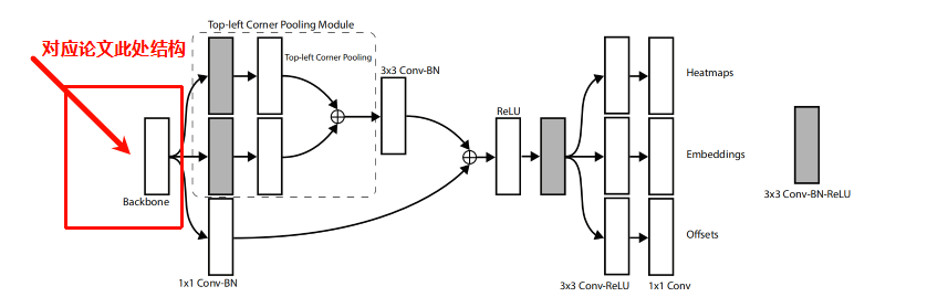
cfg = Config()

角点池化模块

路径一般放在（models/corner_pool.py），模型搭建文件一般放置在此处。

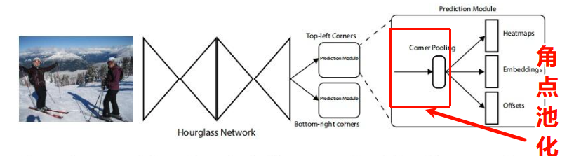
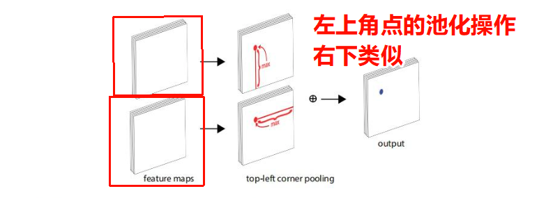
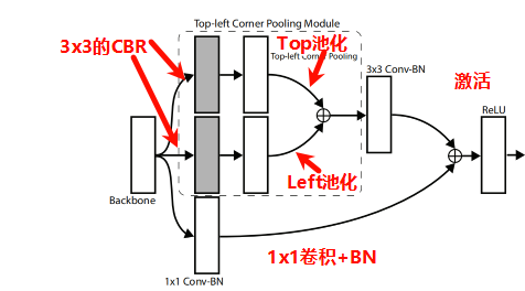
CornerNet将目标的检测问题转换为角点检测问题（左上和右下角点确认了之后，整个目标就确定了）。为此，论文提出了角点池化的操作。一个目标框的角点一般是在目标之外的，不能基于局部特征来定位角点，需要从横向和纵向的方向分别来查找最上面的边界和最左边的边界来定位左上角的角点。这就是corner pooling的灵感。它使用2个特征图，每一个像素位置上，使用第一个特征图向右取得最大的池化特征，使用第二个特征图向下取得最大池化特征，然后再把2个特征向量相加。如下图所示：

首先，我们定义上下左右单一方向的池化类

bash 复制代码

class TopPool(nn.Module):
    "从上到下累计最大值"
    def __init__(self):
        super(TopPool, self).__init__()
    def forward(self, x):
        output,_ = torch.cummax(x, dim=2)
        return output
# 依次可以上下左右都同样的操作
class BottomPool(nn.Module):
    "从下到上累计最大值"
    def __init__(self):
        super(BottomPool, self).__init__()
    def forward(self, x):
        output,_ = torch.cummax(x.flip(2), dim=2)
        return output.flip(2)

class LeftPool(nn.Module):
    "从左往右积累最大值"
    def __init__(self):
        super(LeftPool, self).__init__()
    def forward(self, x):
        output,_ = torch.cummax(x, dim=3)
        return output

class RightPool(nn.Module):
    "从右往左积累最大值"
    def __init__(self):
        super(RightPool, self).__init__()
    def forward(self, x):
        output,_ = torch.cummax(x.flip(3), dim=3)
        return output.flip(3)

把这种池化组合起来，不就是角点的池化操作嘛

py 复制代码

import torch
import torch.nn as nn


class TopPool(nn.Module):
    def forward(self, x: torch.Tensor) -> torch.Tensor:
        out, _ = torch.cummax(x.flip(2), dim=2)
        return out.flip(2)


class BottomPool(nn.Module):
    def forward(self, x: torch.Tensor) -> torch.Tensor:
        out, _ = torch.cummax(x, dim=2)
        return out


class LeftPool(nn.Module):
    def forward(self, x: torch.Tensor) -> torch.Tensor:
        out, _ = torch.cummax(x.flip(3), dim=3)
        return out.flip(3)


class RightPool(nn.Module):
    def forward(self, x: torch.Tensor) -> torch.Tensor:
        out, _ = torch.cummax(x, dim=3)
        return out


class Convolution(nn.Module):
    def __init__(self, k, inp_dim, out_dim, stride=1, padding=None):
        super().__init__()
        if padding is None:
            padding = (k - 1) // 2
        self.conv = nn.Conv2d(inp_dim, out_dim, k, stride=stride, padding=padding, bias=False)
        self.bn = nn.BatchNorm2d(out_dim)
        self.relu = nn.ReLU(inplace=True)

    def forward(self, x):
        return self.relu(self.bn(self.conv(x)))


class CornerPooling(nn.Module):
    """
    CornerNet-style corner pooling block:
      - top_left:  TopPool (down) + LeftPool (right)
      - bottom_right: BottomPool (up) + RightPool (left)
    """
    def __init__(self, in_channels, inter_channels=128, mode="top_left"):
        super().__init__()
        if mode == "top_left":
            self.pool1 = TopPool()
            self.pool2 = LeftPool()
        elif mode == "bottom_right":
            self.pool1 = BottomPool()
            self.pool2 = RightPool()
        else:
            raise ValueError("mode must be 'top_left' or 'bottom_right'.")

        # 官方风格：pool 前 3x3 conv 两分支
        self.p1_conv = Convolution(3, in_channels, inter_channels)
        self.p2_conv = Convolution(3, in_channels, inter_channels)

        # 融合回 in_channels
        self.conv = nn.Sequential(
            nn.Conv2d(inter_channels, in_channels, 3, padding=1, bias=False),
            nn.BatchNorm2d(in_channels),
        )

        # skip 走 1x1 conv（官方常见）
        self.skip = nn.Sequential(
            nn.Conv2d(in_channels, in_channels, 1, bias=False),
            nn.BatchNorm2d(in_channels),
        )
        self.relu = nn.ReLU(inplace=True)

    def forward(self, x):
        p1 = self.pool1(self.p1_conv(x))
        p2 = self.pool2(self.p2_conv(x))
        out = self.conv(p1 + p2)
        return self.relu(out + self.skip(x))

具体图示可以见下图（源于论文原图），右下角点操作类似。

backbone实现

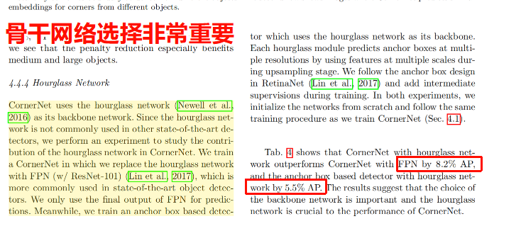
backbone主要是用于特征提取的，选择任何一种backbone都可以（但是原文中好像提到了hourglass是非常重要的，使用hourglass网络的指标最高），角点池化操作在backbone提取特征之后。

对于Hourglass的网络的实现可以使用递归的方式进行

文件路径：Hourglass Network (models/backbone.py)

1）基本卷积块

python 复制代码

class Convolution(nn.Module):
    def __init__(self, k, inp_dim, out_dim, stride=1, padding=None):
        super().__init__()
        if padding is None:
            padding = (k - 1) // 2
        self.conv = nn.Conv2d(inp_dim, out_dim, k, stride=stride, padding=padding, bias=False)
        self.bn = nn.BatchNorm2d(out_dim)
        self.relu = nn.ReLU(inplace=True)

    def forward(self, x):
        return self.relu(self.bn(self.conv(x)))

2）基本残差块

python 复制代码

class Residual(nn.Module):
    def __init__(self, inp_dim, out_dim, stride=1):
        super().__init__()
        self.conv1 = nn.Conv2d(inp_dim, out_dim, 3, stride=stride, padding=1, bias=False)
        self.bn1 = nn.BatchNorm2d(out_dim)
        self.conv2 = nn.Conv2d(out_dim, out_dim, 3, stride=1, padding=1, bias=False)
        self.bn2 = nn.BatchNorm2d(out_dim)
        self.relu = nn.ReLU(inplace=True)

        self.skip = None
        if stride != 1 or inp_dim != out_dim:
            self.skip = nn.Sequential(
                nn.Conv2d(inp_dim, out_dim, 1, stride=stride, bias=False),
                nn.BatchNorm2d(out_dim),
            )

    def forward(self, x):
        residual = x if self.skip is None else self.skip(x)
        out = self.relu(self.bn1(self.conv1(x)))
        out = self.bn2(self.conv2(out))
        return self.relu(out + residual)

3）基本Hourglass模块

首先定义一个残差块函数，由于将残差块儿串起来。

除了第一个会改变尺寸之外，后续的残差块均不改变尺寸。

python 复制代码

#残差层构建函数 
def make_layer(inp_dim, out_dim, num_modules, stride=1):
    # 第一步：创建第一个残差块（唯一可能下采样的块）
    # 作用：如果stride=2，这一步会把特征图尺寸减半、通道数从inp_dim→out_dim
    layers = [Residual(inp_dim, out_dim, stride=stride)]
    # 第二步：创建剩下的num_modules-1个残差块
    # 作用：仅做特征提取，不改变尺寸/通道（stride=1，输入输出都是out_dim）
    for _ in range(1, num_modules):
        layers.append(Residual(out_dim, out_dim, stride=1))
    return nn.Sequential(*layers)

构建hourglass的基础stack,即基本漏斗单位。为了代码简洁，使用递归实现。

python 复制代码

class KPModule(nn.Module):
    def __init__(self, n, dims, modules):
        super().__init__()
        # 校验参数：递归层数n → dims/modules长度必须是n+1（比如n=5→长度6）
        assert len(dims) == n + 1
        assert len(modules) == n + 1

        # 取当前层的通道数/残差块数，以及下一层递归的参数
        curr_dim, next_dim = dims[0], dims[1]  # 比如n=5时：curr_dim=256, next_dim=256
        curr_mod, next_mod = modules[0], modules[1]  # curr_mod=2, next_mod=2

        # 上分支：不改变尺寸/通道，仅提取特征（对应论文的"top branch"）
        self.up1 = make_layer(curr_dim, curr_dim, curr_mod, stride=1)
        
        # 下分支第一步：下采样（尺寸/2）+ 通道升级（比如256→384）
        self.low1 = make_layer(curr_dim, next_dim, curr_mod, stride=2)

        # 递归核心：n>1时，调用自己（套娃）；n=1时，到最底层（无递归）
        if n > 1:
            # 比如n=5→调用KPModule(4, dims[1:], modules[1:]) → 继续套娃
            self.low2 = KPModule(n - 1, dims[1:], modules[1:])
        else:
            # n=1时，最底层：仅用残差块提取特征（对应论文的"bottleneck"）
            self.low2 = make_layer(next_dim, next_dim, next_mod, stride=1)

        # 下分支最后一步：把通道数恢复为当前层的curr_dim（比如384→256）
        self.low3 = make_layer(next_dim, curr_dim, curr_mod, stride=1)

    def forward(self, x):
        # 上分支：提取原尺寸特征
        up1 = self.up1(x)  
        
        # 下分支第一步：下采样，缩小尺寸、升级通道
        low1 = self.low1(x)  
        
        # 下分支第二步：递归处理（套娃），提取全局特征
        low2 = self.low2(low1)  
        
        # 下分支第三步：恢复通道数
        low3 = self.low3(low2)  
        
        # 下分支第四步：上采样，把low3的尺寸放大到和up1一致（最近邻插值，论文指定）
        up2 = F.interpolate(low3, size=up1.shape[-2:], mode="nearest")  
        
        # 特征融合：原尺寸特征 + 多尺度融合特征（核心操作）
        return up1 + up2

最后构建Hourglass104网络

python 复制代码

class Hourglass104(nn.Module):
    """
    CornerNet Hourglass-104 backbone (2-stack default).
    输入 511x511 -> 输出 stride=4 的 128x128 特征（每个 stack 256 通道）。
    """
    def __init__(
        self,
        num_stacks=2,
        n=5,
        dims=(256, 256, 384, 384, 384, 512),
        modules=(2, 2, 2, 2, 2, 4),
    ):
        super().__init__()
        assert len(dims) == n + 1
        assert len(modules) == n + 1

        self.num_stacks = num_stacks
        self.relu = nn.ReLU(inplace=True)

        # 前置处理层（Input Stem）
        # 第1层：7×7卷积 + BN + ReLU，stride=2
        # 参数：k=7, inp_dim=3（输入通道）, out_dim=128（输出通道）, stride=2
        # 效果：尺寸511→256（511//2=255？实际PyTorch会自动补边，最终≈256），通道3→128
        self.pre = nn.Sequential(
            Convolution(7, 3, 128, stride=2),  # 7×7卷积，stride=2 → 尺寸/2
            Residual(128, 256, stride=2),  # 残差下采样 → 尺寸/2（总stride=4）
            Residual(256, 256, stride=1),
            Residual(256, 256, stride=1),
        )

        # 多stack沙漏（默认2个）
        # 多stack沙漏：创建num_stacks个KPModule（默认2个）
			 # nn.ModuleList：专门存储网络层的列表，PyTorch能识别其中的参数（普通list不行）
			 #这样子的话，self.hgs[0]可以调用第一个沙漏，self.hgs[1]调用第二个，且 PyTorch 会自动把这些层的参数加入优化器。
        self.hgs = nn.ModuleList([KPModule(n, list(dims), list(modules)) for _ in range(num_stacks)])
        # 每个沙漏输出后，加一个3×3卷积细化特征（通道不变：256→256）
        self.cnvs = nn.ModuleList([Convolution(3, 256, 256, stride=1) for _ in range(num_stacks)])

        # 多stack之间的特征融合（仅num_stacks>1时）
        if num_stacks > 1:   # 只有当沙漏数量>1时（默认2个），才需要融合
            self.inters_ = nn.ModuleList([
            # 1×1卷积（无偏置） + BN
                nn.Sequential(nn.Conv2d(256, 256, 1, bias=False), nn.BatchNorm2d(256))
                for _ in range(num_stacks - 1)
            ])
            self.cnvs_ = nn.ModuleList([
            # cnvs_：对当前stack的输出做1×1卷积（匹配inters_的维度）
                nn.Sequential(nn.Conv2d(256, 256, 1, bias=False), nn.BatchNorm2d(256))
                for _ in range(num_stacks - 1)
            ])
            # inters：残差块，融合后再细化特征
            self.inters = nn.ModuleList([Residual(256, 256, stride=1) for _ in range(num_stacks - 1)])

    def forward(self, x):
    #第一步：前置处理 → inter的shape=(batch_size, 256, 128, 128)
        inter = self.pre(x)  # 前置处理 → stride=4
        # # 保存每个stack的输出
        outs = []
        for i in range(self.num_stacks):
        # 第二步：第i个沙漏处理inter → hg的shape=(256,128,128)
            hg = self.hgs[i](inter)  # 第i个沙漏
            cnv = self.cnvs[i](hg)  # 沙漏输出后卷积
            outs.append(cnv)
            if i < self.num_stacks - 1:  # 多stack之间特征传递
                inter = self.inters_[i](inter) + self.cnvs_[i](cnv)  # 特征融合
                inter = self.relu(inter)
                inter = self.inters[i](inter)  # 残差处理
        return outs

到此，网络的骨干网络就搭建完毕。即论文中对应的backbone部分。

后续backbone部分提取的特征将会被用于后续的角点池化与热力图图预测。