Deep Learning with PyTorch: A Gentle Introduction to torch.autograd

[1. Background](#1. Background)
[2. Usage in PyTorch](#2. Usage in PyTorch)
[3. Differentiation in Autograd](#3. Differentiation in Autograd)
[4. Computational Graph](#4. Computational Graph)
[5. Exclusion from the DAG](#5. Exclusion from the DAG)
References

A Gentle Introduction to torch.autograd
https://docs.pytorch.org/tutorials/beginner/blitz/autograd_tutorial.html

torch.autograd is PyTorch's automatic differentiation engine that powers neural network training.

复制代码

differentiation [ˌdɪfəˌrenʃɪ'eɪʃn]
n. 区别；区分；分化

1. Background

Neural networks (NNs) are a collection of nested functions that are executed on some input data. These functions are defined by parameters (consisting of weights and biases), which in PyTorch are stored in tensors.

Training a NN happens in two steps:

Forward Propagation : In forward propagation, the NN makes its best guess about the correct output. It runs the input data through each of its functions to make this guess.
Backward Propagation : In backward propagation, the NN adjusts its parameters proportionate to the error in its guess. It does this by traversing backwards from the output, collecting the derivatives of the error with respect to the parameters of the functions (gradients), and optimizing the parameters using gradient descent.

proportionate [prəˈpɔː(r)ʃ(ə)nət]
adj. 成比例的；相应的；相称的
v. 使成比例；使适应
descent [dɪ'sent]
n. 下降；血统；祖先；斜坡

2. Usage in PyTorch

Let's take a look at a single training step. For this example, we load a pretrained resnet18 model from torchvision. We create a random data tensor to represent a single image with 3 channels, and height & width of 64, and its corresponding label initialized to some random values. Label in pretrained models has shape (1,1000).

Note

This tutorial works only on the CPU and will not work on GPU devices (even if tensors are moved to CUDA).

复制代码

import torch
from torchvision.models import resnet18, ResNet18_Weights
model = resnet18(weights=ResNet18_Weights.DEFAULT)
data = torch.rand(1, 3, 64, 64)
labels = torch.rand(1, 1000)

Downloading: "https://download.pytorch.org/models/resnet18-f37072fd.pth" to /var/lib/ci-user/.cache/torch/hub/checkpoints/resnet18-f37072fd.pth

  0%|          | 0.00/44.7M [00:00<?, ?B/s]
 80%|████████  | 35.9M/44.7M [00:00<00:00, 376MB/s]
100%|██████████| 44.7M/44.7M [00:00<00:00, 383MB/s]

Next, we run the input data through the model through each of its layers to make a prediction. This is the forward pass.

复制代码

prediction = model(data)  # forward pass

We use the model's prediction and the corresponding label to calculate the error (loss). The next step is to backpropagate this error through the network. Backward propagation is kicked off when we call .backward() on the error tensor. Autograd then calculates and stores the gradients for each model parameter in the parameter's .grad attribute.

复制代码

kick off
na. (足球) 中线开球；开始 (某种活动)；死；踢脱 (鞋等)

loss = (prediction - labels).sum()
loss.backward() # backward pass

Next, we load an optimizer, in this case SGD with a learning rate of 0.01 and momentum of 0.9. We register all the parameters of the model in the optimizer.

复制代码

optim = torch.optim.SGD(model.parameters(), lr=1e-2, momentum=0.9)

Finally, we call .step() to initiate gradient descent. The optimizer adjusts each parameter by its gradient stored in .grad.

复制代码

optim.step()  # gradient descent

initiate [ɪˈnɪʃieɪt]
v. 开创；开始；提出；制定
adj. 被传授初步知识的；新入会的
n. 被传授初步知识的人；新入会的人

3. Differentiation in Autograd

We create two tensors a and b with requires_grad=True. This signals to autograd that every operation on them should be tracked.

We create another tensor Q from a and b.

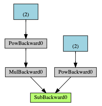
Q = 3 a 3 − b 2 Q = 3a^3 - b^2 Q=3a3−b2

Let's assume a and b to be parameters of an NN, and Q to be the error. In NN training, we want gradients of the error w.r.t. parameters, i.e.

∂ Q ∂ a = 9 a 2 \frac{\partial Q}{\partial a} = 9a^2 ∂a∂Q=9a2
∂ Q ∂ b = − 2 b \frac{\partial Q}{\partial b} = -2b ∂b∂Q=−2b

When we call .backward() on Q, autograd calculates these gradients and stores them in the respective tensors' .grad attribute.

We need to explicitly pass a gradient argument in Q.backward() because it is a vector. gradient is a tensor of the same shape as Q, and it represents the gradient of Q w.r.t. itself, i.e.

d Q d Q = 1 \frac{dQ}{dQ} = 1 dQdQ=1

Equivalently, we can also aggregate Q into a scalar and call backward implicitly, like Q.sum().backward().

复制代码

aggregate [ˈæɡrɪɡeɪt]
n. 骨料；合计；总数
v. 合计；总计
adj. 总数的；总计的

Gradients are now deposited in a.grad and b.grad.

复制代码

# !/usr/bin/env python
# coding=utf-8

import torch
import numpy as np

a = torch.tensor([2., 3.], requires_grad=True)
b = torch.tensor([6., 4.], requires_grad=True)

Q = 3 * a ** 3 - b ** 2
print(f"Q: {Q}")

external_grad = torch.tensor([1., 1.])
Q.backward(gradient=external_grad)

print(9 * a ** 2 == a.grad)
print(-2 * b == b.grad)

print(f"a.grad: {a.grad}")
print(f"b.grad: {b.grad}")

/home/yongqiang/miniconda3/bin/python /home/yongqiang/quantitative_analysis/mse.py 
Q: tensor([-12.,  65.], grad_fn=<SubBackward0>)
tensor([True, True])
tensor([True, True])
a.grad: tensor([36., 81.])
b.grad: tensor([-12.,  -8.])

Process finished with exit code 0

4. Computational Graph

Conceptually, autograd keeps a record of data (tensors) & all executed operations (along with the resulting new tensors) in a directed acyclic graph (DAG) consisting of Function objects. In this DAG, leaves are the input tensors, roots are the output tensors. By tracing this graph from roots to leaves, you can automatically compute the gradients using the chain rule.

In a forward pass, autograd does two things simultaneously:

run the requested operation to compute a resulting tensor, and
maintain the operation's gradient function in the DAG.

The backward pass kicks off when .backward() is called on the DAG root. autograd then:

computes the gradients from each .grad_fn,
accumulates them in the respective tensor's .grad attribute, and
using the chain rule, propagates all the way to the leaf tensors.

Below is a visual representation of the DAG in our example. In the graph, the arrows are in the direction of the forward pass. The nodes represent the backward functions of each operation in the forward pass. The leaf nodes in blue represent our leaf tensors a and b.

Note

DAGs are dynamic in PyTorch

An important thing to note is that the graph is recreated from scratch; after each .backward() call, autograd starts populating a new graph. This is exactly what allows you to use control flow statements in your model; you can change the shape, size and operations at every iteration if needed.

5. Exclusion from the DAG

torch.autograd tracks operations on all tensors which have their requires_grad flag set to True. For tensors that don't require gradients, setting this attribute to False excludes it from the gradient computation DAG.

The output tensor of an operation will require gradients even if only a single input tensor has requires_grad=True.

复制代码

x = torch.rand(5, 5)
y = torch.rand(5, 5)
z = torch.rand((5, 5), requires_grad=True)

a = x + y
print(f"Does `a` require gradients?: {a.requires_grad}")
b = x + z
print(f"Does `b` require gradients?: {b.requires_grad}")

Does `a` require gradients?: False
Does `b` require gradients?: True

In a NN, parameters that don't compute gradients are usually called frozen parameters. It is useful to "freeze" part of your model if you know in advance that you won't need the gradients of those parameters (this offers some performance benefits by reducing autograd computations).

In finetuning, we freeze most of the model and typically only modify the classifier layers to make predictions on new labels. Let's walk through a small example to demonstrate this. As before, we load a pretrained resnet18 model, and freeze all the parameters.

复制代码

from torch import nn, optim

model = resnet18(weights=ResNet18_Weights.DEFAULT)

# Freeze all the parameters in the network
for param in model.parameters():
    param.requires_grad = False

Let's say we want to finetune the model on a new dataset with 10 labels. In resnet, the classifier is the last linear layer model.fc. We can simply replace it with a new linear layer (unfrozen by default) that acts as our classifier.

复制代码

model.fc = nn.Linear(512, 10)

Now all parameters in the model, except the parameters of model.fc, are frozen. The only parameters that compute gradients are the weights and bias of model.fc.

复制代码

# Optimize only the classifier
optimizer = optim.SGD(model.parameters(), lr=1e-2, momentum=0.9)

Notice although we register all the parameters in the optimizer, the only parameters that are computing gradients (and hence updated in gradient descent) are the weights and bias of the classifier.

请注意，虽然我们将所有参数都注册到优化器中，但实际计算梯度 (并在梯度下降过程中进行更新) 的参数只有分类器的权重和偏置。

References

1\] Yongqiang Cheng (程永强), \[2\] Deep Learning with PyTorch: A 60 Minute Blitz, \[3\] Backpropagation calculus,