注:本文为 "傅里叶理论" 相关合辑。
英文引文,机翻未校。
中文引文,略作重排。
如有内容异常,请看原文。
An Introduction to Fourier Theory
傅里叶理论导论
by Forrest M. Hoffman
作者:福雷斯特·M·霍夫曼
Introduction
引言
Linear transforms, especially Fourier and Laplace transforms, are widely used in solving problems in science and engineering. The Fourier transform is used in linear systems analysis, antenna studies, optics, random process modeling, probability theory, quantum physics, and boundary-value problems (Brigham, 2-3) and has been very successfully applied to restoration of astronomical data (Brault and White). The Fourier transform, a pervasive and versatile tool, is used in many fields of science as a mathematical or physical tool to alter a problem into one that can be more easily solved. Some scientists understand Fourier theory as a physical phenomenon, not simply as a mathematical tool. In some branches of science, the Fourier transform of one function may yield another physical function (Bracewell, 1-2).
线性变换,尤其是傅里叶变换和拉普拉斯变换,被广泛应用于解决科学和工程领域的各类问题。傅里叶变换可用于线性系统分析、天线研究、光学、随机过程建模、概率论、量子物理以及边值问题研究(布里格姆,2-3页),并已被极为成功地应用于天文数据的复原工作(布罗特与怀特)。傅里叶变换是一种应用广泛、功能多样的工具,在诸多科学领域中被当作数学或物理工具,将复杂问题转化为更易求解的形式。部分科学家将傅里叶理论视作一种物理现象,而非单纯的数学工具。在一些科学分支中,一个函数的傅里叶变换可能会得到另一个物理函数(布雷思韦尔,1-2页)。
The Fourier Transform
傅里叶变换
The Fourier transform, in essence, decomposes or separates a waveform or function into sinusoids of different frequency which sum to the original waveform. It identifies or distinguishes the different frequency sinusoids and their respective amplitudes (Brigham, 4). The Fourier transform of f ( x ) f(x) f(x) is defined as
傅里叶变换从本质上来说,是将一个波形或函数分解为不同频率的正弦曲线,这些正弦曲线叠加后可还原出原始波形。它能识别并区分不同频率的正弦曲线及其各自的振幅(布里格姆,4页)。函数 f ( x ) f(x) f(x) 的傅里叶变换定义为
F ( s ) = ∫ − ∞ ∞ f ( x ) e − i 2 π x s d x F(s)=\int_{-\infty}^{\infty} f(x) e^{-i 2 \pi x s} d x F(s)=∫−∞∞f(x)e−i2πxsdx
Applying the same transform to F ( s ) F(s) F(s) gives
对 F ( s ) F(s) F(s) 施加相同的变换可得
f ( w ) = ∫ − ∞ ∞ F ( s ) e − i 2 π x s d x . f(w)=\int_{-\infty}^{\infty} F(s) e^{-i 2 \pi x s} d x . f(w)=∫−∞∞F(s)e−i2πxsdx.
If f ( x ) f(x) f(x) is an even function of x, that is f ( x ) = f ( − x ) f(x)=f(-x) f(x)=f(−x) ,then f ( w ) = f ( x ) f(w)=f(x) f(w)=f(x) .If f ( x ) f(x) f(x) is an odd function of x , that is f ( x ) = − f ( − x ) f(x)=-f(-x) f(x)=−f(−x) ,then f ( w ) = f ( − x ) f(w)=f(-x) f(w)=f(−x) .When f ( x ) f(x) f(x) is neither even nor odd, it can often be split into even or odd parts.
若 f ( x ) f(x) f(x) 是关于 x x x 的偶函数,即 f ( x ) = f ( − x ) f(x)=f(-x) f(x)=f(−x) ,则 f ( w ) = f ( x ) f(w)=f(x) f(w)=f(x) ;若 f ( x ) f(x) f(x) 是关于 x x x 的奇函数,即 f ( x ) = − f ( − x ) f(x)=-f(-x) f(x)=−f(−x) ,则 f ( w ) = f ( − x ) f(w)=f(-x) f(w)=f(−x) 。当 f ( x ) f(x) f(x) 既非偶函数也非奇函数时,通常可将其分解为偶部和奇部。
To avoid confusion, it is customary to write the Fourier transform and its inverse so that they exhibit reversibility:
为避免混淆,通常将傅里叶变换及其逆变换写成具有可逆性的形式:
F ( s ) = ∫ − ∞ ∞ f ( x ) e − i 2 π x s d x f ( x ) = ∫ − ∞ ∞ F ( s ) e i 2 π x s d x F(s)=\int_{-\infty}^{\infty} f(x) e^{-i 2 \pi x s} d x\\ f(x)=\int_{-\infty}^{\infty} F(s) e^{i 2 \pi x s} d x F(s)=∫−∞∞f(x)e−i2πxsdxf(x)=∫−∞∞F(s)ei2πxsdx
so that
由此可得
f ( x ) = ∫ − ∞ ∞ ∫ − ∞ ∞ f ( x ) e − i 2 π x s d x e i 2 π x s d s f(x)=\int_{-\infty}^{\infty}\left\\int_{-\\infty}\^{\\infty} f(x) e\^{-i 2 \\pi x s} d x\\right e^{i 2 \pi x s} d s f(x)=∫−∞∞∫−∞∞f(x)e−i2πxsdxei2πxsds
as long as the integral exists and any discontinuities, usually represented by multiple integrals of the form 1 2 f ( x + ) + f ( x − ) \frac{1}{2}f(x_{+})+f(x_{-}) 21f(x+)+f(x−) , are finite. The transform quantity F ( s ) F(s) F(s) is often represented as f ~ ( s ) \tilde{f}(s) f~(s) and the Fourier transform is often represented by the operator F \mathscr{F} F (Bracewell, 6-8).
只要该积分存在,且所有间断点(通常以 1 2 f ( x + ) + f ( x − ) \frac{1}{2}f(x_{+})+f(x_{-}) 21f(x+)+f(x−) 形式的多重积分表示)均为有限值。变换量 F ( s ) F(s) F(s) 常记作 f ~ ( s ) \tilde{f}(s) f~(s) ,傅里叶变换则常以算子 F \mathscr{F} F 表示(布雷思韦尔,6-8页)。
There are functions for which the Fourier transform does not exist; however, most physical functions have a Fourier transform, especially if the transform represents a physical quantity. Other functions can be treated with Fourier theory as limiting cases. Many of the common theoretical functions are actually limiting cases in Fourier theory.
存在一些不存在傅里叶变换的函数,但大多数物理函数都有对应的傅里叶变换,尤其是当该变换代表某一物理量时。其余函数可在傅里叶理论中作为极限情况处理,许多常见的理论函数在傅里叶理论中实际上都是极限情况。
Usually functions or waveforms can be split into even and odd parts as follows
通常,函数或波形可按如下方式分解为偶部和奇部:
f ( x ) = E ( x ) + O ( x ) f(x)=E(x)+O(x) f(x)=E(x)+O(x)
where
其中
E ( x ) = 1 2 f ( x ) + f ( − x ) O ( x ) = 1 2 f ( x ) − f ( − x ) E(x)=\frac{1}{2}f(x)+f(-x)\\1em O(x)=\frac{1}{2}f(x)-f(-x) E(x)=21f(x)+f(−x)O(x)=21f(x)−f(−x)
and E ( x ) E(x) E(x) , O ( x ) O(x) O(x) are, in general, complex. In this representation, the Fourier transform of f ( x ) f(x) f(x) reduces to
且一般情况下, E ( x ) E(x) E(x) 和 O ( x ) O(x) O(x) 为复函数。在该表示形式下, f ( x ) f(x) f(x) 的傅里叶变换可简化为
2 ∫ 0 ∞ E ( x ) c o s ( 2 π x s ) d x − 2 i ∫ 0 ∞ O ( x ) s i n ( 2 π x s ) d x 2 \int_{0}^{\infty} E(x) cos (2 \pi x s) d x-2 i \int_{0}^{\infty} O(x) sin (2 \pi x s) d x 2∫0∞E(x)cos(2πxs)dx−2i∫0∞O(x)sin(2πxs)dx
It follows then that an even function has an even transform and that an odd function has an odd transform. Additional symmetry properties are shown in Table 1 (Bracewell, 14).
由此可推得,偶函数的变换结果为偶函数,奇函数的变换结果为奇函数。更多对称性质如表1所示(布雷思韦尔,14页)。
Table 1: Symmetry Properties of the Fourier Transform
表1:傅里叶变换的对称性质
| function | transform |
|---|---|
| real and even 实且偶 | real and even 实且偶 |
| real and odd 实且奇 | imaginary and odd 虚且奇 |
| imaginary and even 虚且偶 | imaginary and even 虚且偶 |
| complex and even 复且偶 | complex and even 复且偶 |
| complex and odd 复且奇 | complex and odd 复且奇 |
| real and asymmetrical 实且非对称 | complex and asymmetrical 复且非对称 |
| imaginary and asymmetrical 虚且非对称 | complex and asymmetrical 复且非对称 |
| real even plus imaginary odd 实偶部加虚奇部 | real 实 |
| real odd plus imaginary even 实奇部加虚偶部 | imaginary 虚 |
| even 偶 | even 偶 |
| odd 奇 | odd 奇 |
An important case from Table 1 is that of an Hermitian function, one in which the real part is even and the imaginary part is odd, i.e, f ( x ) = f ∗ ( − x ) f(x)=f^{*}(-x) f(x)=f∗(−x) . The Fourier transform of an Hermitian function is even. In addition, the Fourier transform of the complex conjugate of a function f ( x ) f(x) f(x) is F ∗ ( − s ) F^{*}(-s) F∗(−s) , the reflection of the conjugate of the transform.
表1中一种重要的情况是厄米特函数,这类函数的实部为偶函数、虚部为奇函数,即 f ( x ) = f ∗ ( − x ) f(x)=f^{*}(-x) f(x)=f∗(−x) ,其傅里叶变换为偶函数。此外,函数 f ( x ) f(x) f(x) 的复共轭的傅里叶变换为 F ∗ ( − s ) F^{*}(-s) F∗(−s) ,即该函数变换结果的共轭的镜像。
The cosine transform of a function f ( x ) f(x) f(x) is defined as
函数 f ( x ) f(x) f(x) 的余弦变换定义为
F c ( s ) = 2 ∫ 0 ∞ f ( x ) cos 2 π s x d x . F_{c}(s)=2 \int_{0}^{\infty} f(x) \cos 2 \pi s x d x . Fc(s)=2∫0∞f(x)cos2πsxdx.
This is equivalent to the Fourier transform if f ( x ) f(x) f(x) is an even function,. In general, the even part of the Fourier transform of f ( x ) f(x) f(x) is the cosine transform of the even part of f ( x ) f(x) f(x) . The cosine transform has a reverse transform given by
若 f ( x ) f(x) f(x) 为偶函数,其余弦变换与傅里叶变换等价。一般来说, f ( x ) f(x) f(x) 的傅里叶变换的偶部等于其自身偶部的余弦变换。余弦变换的逆变换为
f ( x ) = 2 ∫ 0 ∞ F c ( s ) cos 2 π s x d s . f(x)=2 \int_{0}^{\infty} F_{c}(s) \cos 2 \pi s x d s . f(x)=2∫0∞Fc(s)cos2πsxds.
Likewise, the sine transform of f ( x ) f(x) f(x) is defined by
同理,函数 f ( x ) f(x) f(x) 的正弦变换定义为
F s ( s ) = 2 ∫ 0 ∞ f ( x ) sin 2 π s x d x . F_{s}(s)=2 \int_{0}^{\infty} f(x) \sin 2 \pi s x d x . Fs(s)=2∫0∞f(x)sin2πsxdx.
As a result, i i i times the odd part of the Fourier transform of f ( x ) f(x) f(x) is the sine transform of the odd part of f ( x ) f(x) f(x)
因此, f ( x ) f(x) f(x) 的傅里叶变换的奇部乘以 i i i ,等于其自身奇部的正弦变换。
Combining the sine and cosine transforms of the even and odd parts of f ( x ) f(x) f(x) leads to the Fourier transform of the whole of f ( x ) f(x) f(x) :
将 f ( x ) f(x) f(x) 偶部和奇部的正弦、余弦变换相结合,可得整个 f ( x ) f(x) f(x) 的傅里叶变换:
F f ( x ) = F c E ( x ) − i F s O ( x ) \mathscr{F} f(x)=\mathscr{F}{c} E(x)-i \mathscr{F}{s} O(x) Ff(x)=FcE(x)−iFsO(x)
where F \mathscr{F} F , F c \mathscr{F}{c} Fc ,and F s \mathscr{F}{s} Fs stand for the Fourier transform, the cosine transform, and the sine transform respectively, or
其中 F \mathscr{F} F 、 F c \mathscr{F}{c} Fc 和 F s \mathscr{F}{s} Fs 分别代表傅里叶变换、余弦变换和正弦变换,也可表示为
F ( s ) = 1 2 F c ( s ) − 1 2 i F s ( s ) F(s)=\frac{1}{2} F_{c}(s)-\frac{1}{2} i F_{s}(s) F(s)=21Fc(s)−21iFs(s)
(Bracewell, 17-18).
(布雷思韦尔,17-18页)。
Since the Fourier transform F ( s ) F(s) F(s) is a frequency domain representation of a function f ( x ) f(x) f(x) , the s characterizes the frequency of the decomposed cosinusoids and sinusoids and is equal to the number of cycles per unit of x (Bracewell, 18-21). If a function or waveform is not periodic, then the Fourier transform of the function will be a continuous function of frequency (Brigham,4).
由于傅里叶变换 F ( s ) F(s) F(s) 是函数 f ( x ) f(x) f(x) 在频域的表示形式,变量 s s s 表征分解所得余弦和正弦曲线的频率,其值等于单位 x x x 范围内的周期数(布雷思韦尔,18-21页)。若一个函数或波形非周期函数,那么其傅里叶变换将是关于频率的连续函数(布里格姆,4页)。
The Two Domains
两个域
It is often useful to think of functions and their transforms as occupying two domains. These domains are referred to as the upper and the lower domains in older texts, "as if functions circulated at ground level and their transforms in the underworld" (Bracewell, 135). They are also referred to as the function and transform domains, but in most physics applications they are called the time and frequency domains respectively. Operations performed in one domain have corresponding operations in the other. For example, as will be shown below, the convolution operation in the time domain becomes a multiplication operation in the frequency domain, that is, f ( x ) ⊗ g ( x ) ↔ F ( s ) G ( s ) f(x) \otimes g(x) \leftrightarrow F(s) G(s) f(x)⊗g(x)↔F(s)G(s) . The reverse is also true, F ( s ) ⊗ G ( s ) ↔ f ( x ) g ( x ) F(s) \otimes G(s) \leftrightarrow f(x) g(x) F(s)⊗G(s)↔f(x)g(x) . Such theorems allow one to move between domains so that operations can be performed where they are easiest or most advantageous.
将函数及其变换结果视作分属两个域,这一思路往往十分有用。在早期文献中,这两个域被称为上域和下域,"仿佛函数在地面域存在,而其变换结果在地下域存在"(布雷思韦尔,135页)。它们也被称作函数域和变换域,而在大多数物理应用中,二者分别被称为时域和频域。在一个域中执行的运算,在另一个域中都有对应的运算形式。例如,如下文所示,时域中的卷积运算在频域中变为乘法运算,即 f ( x ) ⊗ g ( x ) ↔ F ( s ) G ( s ) f(x) \otimes g(x) \leftrightarrow F(s) G(s) f(x)⊗g(x)↔F(s)G(s) ;反之亦然, F ( s ) ⊗ G ( s ) ↔ f ( x ) g ( x ) F(s) \otimes G(s) \leftrightarrow f(x) g(x) F(s)⊗G(s)↔f(x)g(x) 。这类定理使得人们可以在两个域之间转换,从而在运算最简便、最有利的域中执行操作。
Fourier Transform Properties
傅里叶变换的性质
Scaling Property
尺度变换性质
If F { f ( x ) } = F ( s ) \mathscr{F}\{f(x)\}=F(s) F{f(x)}=F(s) and a is a real, nonzero constant, then
若 F { f ( x ) } = F ( s ) \mathscr{F}\{f(x)\}=F(s) F{f(x)}=F(s) ,且 a a a 为非零实常数,则
F { f ( a x ) } = ∫ − ∞ ∞ f ( a x ) e − i 2 π s x d x = 1 ∣ a ∣ ∫ − ∞ ∞ f ( β ) e − i 2 π s a β d β = 1 ∣ a ∣ F ( s a ) . \begin{aligned} \mathscr{F}\{f(a x)\} & =\int_{-\infty}^{\infty} f(a x) e^{-i 2 \pi s x} d x \\ & =\frac{1}{|a|} \int_{-\infty}^{\infty} f(\beta) e^{-i 2 \pi \frac{s}{a} \beta} d \beta \\ & =\frac{1}{|a|} F\left(\frac{s}{a}\right) . \end{aligned} F{f(ax)}=∫−∞∞f(ax)e−i2πsxdx=∣a∣1∫−∞∞f(β)e−i2πasβdβ=∣a∣1F(as).
From this, the time scaling property, it is evident that if the width of a function is decreased while its height is kept constant, then its Fourier transform becomes wider and shorter. If its width is increased, its transform becomes narrower and taller.
由这一时域尺度变换性质可明显看出,若保持函数的高度不变、减小其宽度,其傅里叶变换的结果会变得更宽更矮;若增大函数的宽度,其变换结果则会变得更窄更高。
A similar frequency scaling property is given by
与之类似,频域尺度变换性质为
F { 1 ∣ a ∣ f ( x a ) } = F ( a s ) . \mathscr{F}\left\{\frac{1}{|a|} f\left(\frac{x}{a}\right)\right\}=F(a s) . F{∣a∣1f(ax)}=F(as).
Shifting Property
平移性质
If F { f ( x ) } = F ( s ) \mathscr{F}\{f(x)\}=F(s) F{f(x)}=F(s) and x 0 x_{0} x0 is a real constant, then
若 F { f ( x ) } = F ( s ) \mathscr{F}\{f(x)\}=F(s) F{f(x)}=F(s) ,且 x 0 x_{0} x0 为实常数,则
F { f ( x − x 0 ) } = ∫ − ∞ ∞ f ( x − x 0 ) e − i 2 π s x d x = ∫ − ∞ ∞ f ( β ) e − i 2 π s ( β + x 0 ) d β = e − i 2 π x 0 s ∫ − ∞ ∞ f ( β ) e − i 2 π s β d β = F ( s ) e − i 2 π x 0 s . \begin{aligned} \mathscr{F}\left\{f\left(x-x_{0}\right)\right\} & =\int_{-\infty}^{\infty} f\left(x-x_{0}\right) e^{-i 2 \pi s x} d x \\ & =\int_{-\infty}^{\infty} f(\beta) e^{-i 2 \pi s\left(\beta+x_{0}\right)} d \beta \\ & =e^{-i 2 \pi x_{0} s} \int_{-\infty}^{\infty} f(\beta) e^{-i 2 \pi s \beta} d \beta \\ & =F(s) e^{-i 2 \pi x_{0} s} . \end{aligned} F{f(x−x0)}=∫−∞∞f(x−x0)e−i2πsxdx=∫−∞∞f(β)e−i2πs(β+x0)dβ=e−i2πx0s∫−∞∞f(β)e−i2πsβdβ=F(s)e−i2πx0s.
This time shifting property states that the Fourier transform of a shifted function is just the transform of the unshifted function multiplied by an exponential factor having a linear phase.
这一时域平移性质表明,经平移后的函数的傅里叶变换,等于原函数的傅里叶变换乘以一个具有线性相位的指数因子。
Likewise, the frequency shifting property states that if F ( s ) F(s) F(s) is shifted by a constant s 0 s_{0} s0 its inverse transform is multiplied by e i 2 π x s 0 e^{i 2 \pi x s_{0}} ei2πxs0
同理,频域平移性质表明,若将 F ( s ) F(s) F(s) 沿频轴平移常数 s 0 s_{0} s0 ,其逆变换结果等于原函数乘以 e i 2 π x s 0 e^{i 2 \pi x s_{0}} ei2πxs0 ,即
F { f ( x ) e i 2 π x s 0 } = F ( s − s 0 ) . \mathscr{F}\left\{f(x) e^{i 2 \pi x s_{0}}\right\}=F\left(s-s_{0}\right) . F{f(x)ei2πxs0}=F(s−s0).
Convolution Theorem
卷积定理
We now derive the aforementioned time convolution theorem. Suppose that g ( x ) = f ( x ) ⊗ h ( x ) g(x)=f(x) \otimes h(x) g(x)=f(x)⊗h(x) . Then, given that F { g ( x ) } = G ( s ) \mathscr{F}\{g(x)\}=G(s) F{g(x)}=G(s) , F { f ( x ) } = F ( s ) \mathscr{F}\{f(x)\}=F(s) F{f(x)}=F(s) ,and F { h ( x ) } = H ( s ) \mathscr{F}\{h(x)\}=H(s) F{h(x)}=H(s) ,
接下来推导上述的时域卷积定理。设 g ( x ) = f ( x ) ⊗ h ( x ) g(x)=f(x) \otimes h(x) g(x)=f(x)⊗h(x) ,且已知 F { g ( x ) } = G ( s ) \mathscr{F}\{g(x)\}=G(s) F{g(x)}=G(s) 、 F { f ( x ) } = F ( s ) \mathscr{F}\{f(x)\}=F(s) F{f(x)}=F(s) 、 F { h ( x ) } = H ( s ) \mathscr{F}\{h(x)\}=H(s) F{h(x)}=H(s) ,则
G ( s ) = F { f ( x ) ⊗ h ( x ) } = F { ∫ − ∞ ∞ f ( β ) h ( x − β ) d β } = ∫ − ∞ ∞ ∫ − ∞ ∞ f ( β ) h ( x − β ) d β e − i 2 π s x d x = ∫ − ∞ ∞ f ( β ) ∫ − ∞ ∞ h ( x − β ) e − i 2 π s x d x d β = H ( s ) ∫ − ∞ ∞ f ( β ) e − i 2 π s β d β = F ( s ) H ( s ) . \begin{aligned} G(s) & =\mathscr{F}\{f(x) \otimes h(x)\} \\ & =\mathscr{F}\left\{\int_{-\infty}^{\infty} f(\beta) h(x-\beta) d \beta\right\} \\ & =\int_{-\infty}^{\infty}\left\\int_{-\\infty}\^{\\infty} f(\\beta) h(x-\\beta) d \\beta\\right e^{-i 2 \pi s x} d x \\ & =\int_{-\infty}^{\infty} f(\beta)\left\\int_{-\\infty}\^{\\infty} h(x-\\beta) e\^{-i 2 \\pi s x} d x\\right d \beta \\ & =H(s) \int_{-\infty}^{\infty} f(\beta) e^{-i 2 \pi s \beta} d \beta \\ & =F(s) H(s) . \end{aligned} G(s)=F{f(x)⊗h(x)}=F{∫−∞∞f(β)h(x−β)dβ}=∫−∞∞∫−∞∞f(β)h(x−β)dβe−i2πsxdx=∫−∞∞f(β)∫−∞∞h(x−β)e−i2πsxdxdβ=H(s)∫−∞∞f(β)e−i2πsβdβ=F(s)H(s).
This extremely powerful result demonstrates that the Fourier transform of a convolution is simply given by the product of the individual transforms, that is
这一极具实用性的结论表明,卷积的傅里叶变换等于各函数傅里叶变换的乘积,即
F { f ( x ) ⊗ h ( x ) } = F ( s ) H ( s ) . \mathscr{F}\{f(x) \otimes h(x)\}=F(s) H(s) . F{f(x)⊗h(x)}=F(s)H(s).
Using a similar derivation, it can be shown that the Fourier transform of a product is given by the convolution of the individual transforms, that is
F { f ( x ) h ( x ) } = F ( s ) ⊗ H ( s ) . \mathscr{F}\{f(x) h(x)\}=F(s) \otimes H(s) . F{f(x)h(x)}=F(s)⊗H(s).
通过类似的推导过程可证明,函数乘积的傅里叶变换等于各函数傅里叶变换的卷积,即
F { f ( x ) h ( x ) } = F ( s ) ⊗ H ( s ) . \mathscr{F}\{f(x) h(x)\}=F(s) \otimes H(s) . F{f(x)h(x)}=F(s)⊗H(s).
This is the statement of the frequency convolution theorem (Gaskill, 194-197; Brigham, 60-65).
这就是频域卷积定理的表述(加斯基尔,194-197页;布里格姆,60-65页)。
Correlation Theorem
相关定理
The correlation integral, like the convolution integral, is important in theoretical and practical applications. The correlation integral is defined as
相关积分与卷积积分类似,在理论和实际应用中都具有重要意义。相关积分的定义为
h ( x ) = ∫ − ∞ ∞ f ( u ) g ( x + u ) d u h(x)=\int_{-\infty}^{\infty} f(u) g(x+u) d u h(x)=∫−∞∞f(u)g(x+u)du
and like the convolution integral, it forms a Fourier transform pair given by
和卷积积分一样,相关积分也构成一对傅里叶变换,即
F { h ( x ) } = F ( s ) G ∗ ( s ) . \mathscr{F}\{h(x)\}=F(s) G^{*}(s) . F{h(x)}=F(s)G∗(s).
This is the statement of the correlation theorem. If f ( x ) f(x) f(x) and g ( x ) g(x) g(x) are the same function, the integral above is normally called the autocorrelation function, and the crosscorrelation if they differ (Brigham, 65-69). The Fourier transform pair for the autocorrelation is simply
这就是相关定理的表述。若 f ( x ) f(x) f(x) 和 g ( x ) g(x) g(x) 为同一函数,上述积分通常被称为自相关函数;若二者为不同函数,则称为互相关函数(布里格姆,65-69页)。自相关的傅里叶变换对为
F { ∫ − ∞ ∞ f ( u ) f ( x + u ) d u } = ∣ F ∣ 2 . \mathscr{F}\left\{\int_{-\infty}^{\infty} f(u) f(x+u) d u\right\}=|F|^{2} . F{∫−∞∞f(u)f(x+u)du}=∣F∣2.
Parseval's Theorem
帕塞瓦尔定理
Parseval's Theorem states that the power of a signal represented by a function h ( t ) h(t) h(t) is the same whether computed in signal space or frequency (transform) space; that is,
帕塞瓦尔定理指出,由函数 h ( t ) h(t) h(t) 表示的信号的功率,在信号域(时域)和频域(变换域)中计算的结果相等,即
∫ − ∞ ∞ h 2 ( t ) d t = ∫ − ∞ ∞ ∣ H ( f ) ∣ 2 d f \int_{-\infty}^{\infty} h^{2}(t) d t=\int_{-\infty}^{\infty}|H(f)|^{2} d f ∫−∞∞h2(t)dt=∫−∞∞∣H(f)∣2df
(Brigham, 23). The power spectrum, P ( f ) P(f) P(f) , is given by
(布里格姆,23页)。功率谱 P ( f ) P(f) P(f) 的定义为
P ( f ) = ∣ H ( f ) ∣ 2 , − ∞ ≤ f ≤ + ∞ . P(f)=|H(f)|^{2},-\infty \leq f \leq+\infty . P(f)=∣H(f)∣2,−∞≤f≤+∞.
Sampling Theorem
采样定理
A bandlimited signal is a signal, f ( t ) f(t) f(t) , which has no spectral components beyond a frequency B Hz; that is, F ( s ) = 0 F(s)=0 F(s)=0 for ∣ s ∣ > 2 π B |s|>2 \pi B ∣s∣>2πB . The sampling theorem states that a real signal, f ( t ) f(t) f(t) , which is bandlimited to B Hz can be reconstructed without error from samples taken uniformly at a rate R > 2 B R>2 B R>2B samples per second. This minimum sampling frequency, F s = 2 B F_{s}=2 B Fs=2B Hz, is called the Nyquist rate or the Nyquist frequency. The corresponding sampling interval, T = 1 2 B T=\frac{1}{2 B} T=2B1 (where t = n T t=n T t=nT ), is called the Nyquist interval. A signal bandlimited to B Hz which is sampled at less than the Nyquist frequency of 2 B 2 B 2B , i.e., which was sampled at an interval T > 1 2 B T>\frac{1}{2 B} T>2B1 , is said to be undersampled.
带限信号是指不存在频率高于 B B B 赫兹的频谱分量的信号 f ( t ) f(t) f(t) ,即当 ∣ s ∣ > 2 π B |s|>2 \pi B ∣s∣>2πB 时, F ( s ) = 0 F(s)=0 F(s)=0 。采样定理指出,带宽限制在 B B B 赫兹的实信号 f ( t ) f(t) f(t) ,可由以 R > 2 B R>2B R>2B 次/秒的速率均匀采集的样本无误差地重建。这一最低采样频率 F s = 2 B F_{s}=2B Fs=2B 赫兹被称为奈奎斯特速率或奈奎斯特频率,对应的采样间隔 T = 1 2 B T=\frac{1}{2 B} T=2B1 (其中 t = n T t=n T t=nT )被称为奈奎斯特间隔。若对带宽为 B B B 赫兹的带限信号的采样频率低于奈奎斯特频率 2 B 2B 2B ,即采样间隔 T > 1 2 B T>\frac{1}{2 B} T>2B1 ,则称该信号被欠采样。
Aliasing
混叠
A number of practical difficulties are encountered in reconstructing a signal from its samples. The sampling theorem assumes that a signal is bandlimited. In practice, however, signals are timelimited, not bandlimited. As a result, determining an adequate sampling frequency which does not lose desired information can be difficult. When a signal is undersampled, its spectrum has overlapping tails; that is F ( s ) F(s) F(s) no longer has complete information about the spectrum and it is no longer possible to recover f ( t ) f(t) f(t) from the sampled signal. In this case, the tailing spectrum does not go to zero, but is folded back onto the apparent spectrum. This inversion of the tail is called spectral folding or aliasing (Lathi, 532-535).
从信号样本重建原始信号的过程中会遇到诸多实际问题。采样定理的前提是信号为带限信号,但在实际应用中,信号均为时限信号,而非带限信号。因此,确定一个能保证不丢失有效信息的合适采样频率存在一定难度。当信号被欠采样时,其频谱的尾部会发生重叠,即 F ( s ) F(s) F(s) 不再包含完整的频谱信息,此时无法从采样信号中恢复出原始信号 f ( t ) f(t) f(t) 。在这种情况下,频谱的尾部不会趋于零,而是会折叠到表观频谱上,这种尾部的反转现象被称为频谱折叠或混叠(拉西,532-535页)。
As an example, Figure 1 shows a unit gaussian curve sampled at three different rates. The FFT (or Fast Fourier Transform) of the undersampled gaussian appears flattened and its tails do not reach zero. This is a result of aliasing. Additional spectral components have been folded back onto the ends of the spectrum or added to the edges to produce this curve.
如图1所示,以三种不同速率对单位高斯曲线进行采样,欠采样后的高斯曲线的快速傅里叶变换(FFT)结果呈现出扁平化的特征,且其尾部无法趋于零,这就是混叠导致的结果。额外的频谱分量被折叠到频谱的末端,或叠加到频谱的边缘,最终形成了这样的曲线。
Figure 1 was generated using IDL with the following code:
1 !P.Multi=0,3.2
2 a=gauss (256,2.0,2); undersampled
3 fa=fft(a,-1)
4 b=gauss (256,2.0,0.1); oversampled
5 fb=fft(b,-1)
6 c=gauss (256,2.0,0.8) ; critically sampled
7 fc=fft(c,-1)
8 plot,a,title='Undersampled Gaussian'
9 plot,b,title='Oversampled Gaussian'
10 plot,c,title='Critically-Sampled Gaussian'
11 plot,shift(abs(fa), 128), title='FFT of Undersampled Gaussian'
12 plot,shift(abs(fb),128),title='FFT of Oversampled Gaussian'
13 plot,shift(abs(fc), 128),title='FFT of Critically-Sampled Gaussian'
图 1 是通过 IDL 语言编写以下代码生成的:
1 !P.Multi=0,3.2
2 a=gauss (256,2.0,2); 欠采样
3 fa=fft(a,-1)
4 b=gauss (256,2.0,0.1); 过采样
5 fb=fft(b,-1)
6 c=gauss (256,2.0,0.8) ; 临界采样
7 fc=fft(c,-1)
8 plot,a,title='欠采样高斯曲线'
9 plot,b,title='过采样高斯曲线'
10 plot,c,title='临界采样高斯曲线'
11 plot,shift(abs(fa), 128), title='欠采样高斯曲线的快速傅里叶变换'
12 plot,shift(abs(fb),128),title='过采样高斯曲线的快速傅里叶变换'
13 plot,shift(abs(fc), 128),title='临界采样高斯曲线的快速傅里叶变换'
The FFT of the oversampled gaussian reaches zero very quickly. Much of its spectrum is zero and is not needed to reconstruct the original gaussian.
过采样后的高斯曲线的快速傅里叶变换结果会迅速趋于零,其频谱的大部分区域值均为零,这些部分对于重建原始高斯曲线并非必需。
Finally, the FFT of the critically-sampled gaussian has tails which reach zero at their ends. The data in the spectrum of the critically-sampled gaussian is just sufficient to reconstruct the original. This gaussian was sampled at the Nyquist frequency.
而临界采样后的高斯曲线的快速傅里叶变换结果,其尾部在末端恰好趋于零,该频谱中的数据量刚好足以重建原始高斯曲线,这种采样方式采用的是奈奎斯特频率。
The gauss function is as follows:
function gauss,dim, fwhm, interval
; points with a full width at half maximum of fwhm sampled with a periodicity of interval
; dim = the number of points
; interval = sampling interval
; fwhm = full width half max of gaussian
center=dim/2.0 ; automatically center gaussian in dim points
x=findgen(dim)-center
sigma=fwhm/sqrt(8.0 * alog(2.0)); fwhm is in data points
coeff=1.0/( sqrt(2.0*!Pi)(sigma/interval))
data=coeff * exp( -(interval * x)^2.0/ (2.0 sigma^2.0))
return,data
end
上述代码中的g auss 函数定义如下:
function gauss,dim, fwhm, interval
; 对半高全宽为fwhm的高斯曲线,以interval为采样间隔进行采样
; dim = 采样点数
; interval = 采样间隔
; fwhm = 高斯曲线的半高全宽
center=dim/2.0 ; 将高斯曲线自动居中于dim个采样点中
x=findgen(dim)-center
sigma=fwhm/sqrt(8.0 * alog(2.0)); 半高全宽的单位为数据点
coeff=1.0/( sqrt(2.0*!Pi)(sigma/interval))
data=coeff * exp( -(interval * x)^2.0/ (2.0 sigma^2.0))
return,data
end
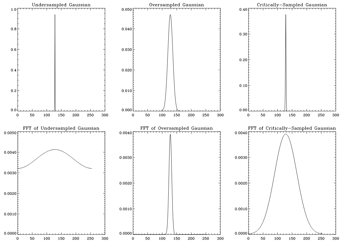
Figure 1: Undersampled, oversampled, and critically-sampled unit area gaussian curves.
图 1:单位面积高斯曲线的欠采样、过采样和临界采样结果
Discrete Fourier Transform (DFT)
离散傅里叶变换(DFT)
Because a digital computer works only with discrete data, numerical computation of the Fourier transform of f ( t ) f(t) f(t) requires discrete sample values of f ( t ) f(t) f(t) , which we will call f k f_{k} fk .In addition, a computer can compute the transform F ( s ) F(s) F(s) only at discrete values of s , that is, it can only provide discrete samples of the transform, F r F_{r} Fr .If f ( k T ) f(k T) f(kT) and F ( r s 0 ) F(r s_{0}) F(rs0) are the k t h k th kth and r t h rth rth samples of f ( t ) f(t) f(t) and F ( s ) F(s) F(s) ,respectively, and N 0 N_{0} N0 is the number of samples in the signal in one period T 0 T_{0} T0 , then
由于数字计算机仅能处理离散数据,对 f ( t ) f(t) f(t) 进行傅里叶变换的数值计算时,需要获取 f ( t ) f(t) f(t) 的离散样本值,记为 f k f_{k} fk 。此外,计算机仅能在离散的 s s s 值处计算变换结果 F ( s ) F(s) F(s) ,即只能得到变换结果的离散样本 F r F_{r} Fr 。若 f ( k T ) f(k T) f(kT) 和 F ( r s 0 ) F(r s_{0}) F(rs0) 分别为 f ( t ) f(t) f(t) 和 F ( s ) F(s) F(s) 的第 k k k 个和第 r r r 个样本,且 N 0 N_{0} N0 为信号在一个周期 T 0 T_{0} T0 内的采样点数,则
f k = T f ( k T ) = T 0 N 0 f ( k T ) f_{k}=T f(k T)=\frac{T_{0}}{N_{0}} f(k T) fk=Tf(kT)=N0T0f(kT)
and
且
F r = F ( r s 0 ) F_{r}=F\left(r s_{0}\right) Fr=F(rs0)
where
其中
s 0 = 2 π F 0 = 2 π T 0 s_{0}=2 \pi F_{0}=\frac{2 \pi}{T_{0}} s0=2πF0=T02π
The discrete Fourier transform (DFT) is defined as
离散傅里叶变换(DFT)的定义为
F r = ∑ k = 0 N 0 − 1 f k e − i r Ω 0 k F_{r}=\sum_{k=0}^{N_{0}-1} f_{k} e^{-i r \Omega_{0} k} Fr=k=0∑N0−1fke−irΩ0k
where Ω 0 = 2 π N 0 \Omega_{0}=\frac{2 \pi}{N_{0}} Ω0=N02π .Its inverse is
其中 Ω 0 = 2 π N 0 \Omega_{0}=\frac{2 \pi}{N_{0}} Ω0=N02π ,其逆变换为
f k = 1 N 0 ∑ r = 0 N 0 − 1 F r e i r Ω 0 k f_{k}=\frac{1}{N_{0}} \sum_{r=0}^{N_{0}-1} F_{r} e^{i r \Omega_{0} k} fk=N01r=0∑N0−1FreirΩ0k
These equations can be used to compute transforms and inverse transforms of appropriately sampled data. Proofs of these relationships are in Lathi (546-548).
上述公式可用于对经过适当采样的数据进行变换和逆变换计算,这些关系式的证明可参见拉西的著作(546-548页)。
Fast Fourier Transform (FFT)
快速傅里叶变换(FFT)
The Fast Fourier Transform (FFT) is a DFT algorithm developed by Tukey and Cooley in 1965 which reduces the number of computations from something on the order of N 0 2 N_{0}^{2} N02 to N 0 log N 0 N_{0} \log N_{0} N0logN0 . There are basically two types of Tukey-Cooley FFT algorithms in use: decimation-in-time and decimation-in-frequency. The algorithm is simplified if N 0 N_{0} N0 is chosen to be a power of 2, but it is not a requirement.
快速傅里叶变换(FFT)是由图基和库利在1965年提出的一种离散傅里叶变换算法,该算法将离散傅里叶变换的计算量从 N 0 2 N_{0}^{2} N02 量级降低至 N 0 log N 0 N_{0} \log N_{0} N0logN0 量级。目前常用的图基-库利快速傅里叶变换算法主要有两种:时域抽取法和频域抽取法。若将采样点数 N 0 N_{0} N0 选为2的幂次,可简化该算法的计算过程,但这并非算法的强制要求。
Summary
总结
The Fourier transform, an invaluable tool in science and engineering, has been introduced and defined. Its symmetry and computational properties have been described and the significance of the time or signal space (or domain) vs. the frequency or spectral domain has been mentioned. In addition, important concepts in sampling required for the understanding of the sampling theorem and the problem of aliasing have been discussed. An example of aliasing was provided along with a short description of the discrete Fourier transform (DFT) and its popular offspring, the Fast Fourier Transform (FFT) algorithm.
本文对傅里叶变换这一科学和工程领域的重要工具进行了介绍和定义,阐述了其对称性质和运算性质,同时说明了时域(信号域)和频域(谱域)的重要意义。此外,本文还探讨了理解采样定理和混叠问题所需的各类重要采样概念,给出了混叠现象的实例,并简要介绍了离散傅里叶变换(DFT)及其应用广泛的改进算法------快速傅里叶变换(FFT)算法。
References
参考文献
- Blass, William E. and Halsey, George W., 1981, Deconvolution of Absorption Spectra, New York: Academic Press, 158 pp.
布拉斯·威廉·E、哈尔西·乔治·W,1981年,《吸收光谱的解卷积》,纽约:学术出版社,158页。 - Bracewell, Ron N., 1965, The Fourier Transform and Its Applications, New York: McGraw-Hill Book Company, 381 pp.
布雷思韦尔·罗恩·N,1965年,《傅里叶变换及其应用》,纽约:麦格劳-希尔图书公司,381页。 - Brault, J. W. and White, O. R., 1971, The analysis and restoration of astronomical data via the fast Fourier transform, Astron. Astrophys., 13, pp.169-189.
布罗特·J·W、怀特·O·R,1971年,《基于快速傅里叶变换的天文数据分析与复原》,《天体物理学杂志》,第13卷,169-189页。 - Brigham, E. Oren, 1988, The Fast Fourier Transform and Its Applications, Englewood Cliffs, NJ: Prentice-Hall, Inc., 448 pp.
布里格姆·E·奥伦,1988年,《快速傅里叶变换及其应用》,新泽西州恩格尔伍德克利夫斯:普伦蒂斯-霍尔出版公司,448页。 - Cooley, J. W, and Tukey, J. W., 1965, An algorithm for the machine calculation of complex Fourier series, Mathematics of Computation, 19, 90, pp. 297-301.
库利·J·W、图基·J·W,1965年,《复傅里叶级数的机器计算算法》,《计算数学》,第19卷第90期,297-301页。 - Gabel, Robert A. and Roberts, Richard A., 1973, Signals and Linear Systems, New York: John Wiley & Sons, 415 pp.
加贝尔·罗伯特·A、罗伯茨·理查德·A,1973年,《信号与线性系统》,纽约:约翰·威利父子出版公司,415页。 - Gaskill, Jack D., 1978, Linear Systems, Fourier Transforms, and Optics, New York: John Wiley & Sons, 554 pp.
加斯基尔·杰克·D,1978年,《线性系统、傅里叶变换与光学》,纽约:约翰·威利父子出版公司,554页。 - Lathi, B. P., 1992, Linear Systems and Signals, Carmichael, Calif: Berkeley-Cambridge Press, 656 pp.
拉西·B·P,1992年,《线性系统与信号》,加利福尼亚州卡迈克尔:伯克利-剑桥出版社,656页。
傅里叶变换原理
Rain 发表于 2024-03-08 | 更新于 2024-04-22
1 连续与离散信号
通常所提及的傅里叶变换均指向连续傅里叶变换(Continuous Fourier Transform, CFT),该变换的处理对象为连续时域信号。
1.1 连续信号
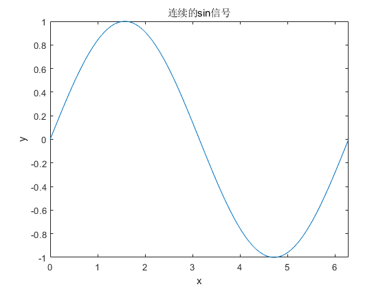
根据维基百科定义,连续信号 (或称连续时间信号)是定义在实数域的信号,其自变量(一般为时间)的取值呈连续特征;若信号的幅值与自变量均连续,则该信号为模拟信号。基于实数的性质,时间参数的连续性意味着信号在时间的任意取值点均有定义。
对于一个正弦函数的连续信号,其波形如下图所示:
1.2 离散信号
对于计算设备的信号处理过程,因采样设备的采样率存在有限性,所获取的采样信号均为离散信号,由此衍生出针对离散信号的离散傅里叶变换(Discrete Fourier Transform, DFT)。
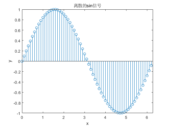
维基百科对离散信号的定义为:离散信号是对连续信号进行采样后得到的信号。与连续信号自变量的连续特性不同,离散信号表现为一个序列,其自变量呈"离散"特征,该序列的每个取值均可视为连续信号的一个采样值。由于离散信号仅为采样序列,无法从中获取采样率,因此采样率需单独存储。以时间为自变量的离散信号称为离散时间信号。
离散信号与数字信号并非同一概念 :数字信号不仅满足自变量的离散性,其幅值还经过量化处理,即自变量与幅值均为离散值。因此,离散信号的精度可以是无限的,而数字信号的精度存在有限性;取值连续、具备无限精度的离散信号被称为抽样信号。离散信号包含数字信号与抽样信号两类。
2 傅里叶变换公式及实际意义
2.1 连续傅里叶变换基本公式
连续傅里叶变换的数学表达式为:
F ( ω ) = ∫ − ∞ ∞ f ( t ) e − j ω t d t F(\omega) = \int_{-\infty}^{\infty} f(t) \, e^{-j\omega t} \, \mathrm{d}t F(ω)=∫−∞∞f(t)e−jωtdt
式中:
- f ( t ) f(t) f(t) 为频谱未知的时域信号,是傅里叶变换的处理对象;
- F ( ω ) F(\omega) F(ω) 为傅里叶变换后的频谱函数,其自变量 ω \omega ω 为角频率;
- e − j ω t e^{-j\omega t} e−jωt 为复指数信号。
2.2 复指数信号的三角形式转换
复指数信号可通过欧拉公式转换为三角函数形式:
e − j ω t = cos ( ω t ) − j sin ( ω t ) e^{-j\omega t} = \cos(\omega t) - j\sin(\omega t) e−jωt=cos(ωt)−jsin(ωt)
将上式代入连续傅里叶变换基本公式,可得展开形式:
F ( ω ) = ∫ − ∞ ∞ f ( t ) cos ( ω t ) − j sin ( ω t ) d t F(\omega) = \int_{-\infty}^{\infty} f(t) \left \\cos(\\omega t) - j\\sin(\\omega t) \\right \mathrm{d}t F(ω)=∫−∞∞f(t)cos(ωt)−jsin(ωt)dt
由该展开式可知,获取信号的频域与相位信息,需将时域信号与复指数信号相乘后进行积分运算。
2.3 信号的频率筛选原理
傅里叶变换的基本实现逻辑为信号的频率筛选,其过程可通过"基信号与未知信号相乘后积分"的方式实现。取已知频率的正弦/余弦基信号,与频谱未知的时域信号进行逐点相乘,再对相乘结果做积分运算。
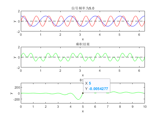
按照傅里叶变换公式所描述的方法,将信号与各频率基信号相乘后积分,MATLAB 仿真结果如下图所示:
图示说明:
- 框图 1 内蓝色信号线为 MATLAB 生成需要做傅里叶变换的随机频率信号(未知信号),红色信号线为频率不断增大的正弦信号(基信号),其频率已知;
- 框图 2 为两正弦波相乘结果;
- 框图 3 是对正弦波乘积结果的积分。
从图中可以直观看出,当未知信号与基信号频率相同时,二者乘积的积分达到最大值。该现象的本质为:当基信号与未知信号频率完全一致时,二者时域相乘的结果整体呈正数值(利用乘法"负负得正"的特性),积分运算后得到的累加值达到峰值。
通过遍历不同频率的基信号,即可确定未知信号中包含的频率成分,其数学表达为:
F ( ω ) = ∫ − ∞ ∞ f ( t ) sin ( ω t ) d t F(\omega) = \int_{-\infty}^{\infty} f(t) \sin(\omega t) \, \mathrm{d}t F(ω)=∫−∞∞f(t)sin(ωt)dt
上述表达式与标准傅里叶变换公式已具有相似形式。
对于包含多个频率成分的复合信号,该筛选方法同样适用:
遍历不同频率的基信号,与复合信号完成"相乘-积分"操作后,积分结果的峰值位置将与复合信号中的各频率成分一一对应,从而实现多频率成分的提取。
3 初始相位对频率筛选的影响
上述频率筛选过程的推导均建立在未知信号初始相位为 0 0 0 的前提条件下。在实际工程应用中,信号的频率与初始相位均为未知量,若仅采用单一正弦或余弦基信号进行"相乘-积分"操作,会因初始相位的非零特性导致频率筛选结果出现偏差,如下图所示:
针对该问题,傅里叶变换采用复指数信号 e − j ω t = cos ( ω t ) − j sin ( ω t ) e^{-j\omega t} = \cos(\omega t) - j\sin(\omega t) e−jωt=cos(ωt)−jsin(ωt) 替代单一三角函数基信号,将未知信号与复指数信号相乘后积分。傅里叶变换的结果为复数,其实部值表征未知信号与余弦基信号的相关度,虚部值表征未知信号与正弦基信号的相关度。因此,傅里叶变换的结果可同时反映未知信号的频率与相位信息。
为单独提取信号的频率信息,需对傅里叶变换的复数结果做模值运算:
∣ F ( ω ) ∣ = { R e F ( ω ) } 2 + { I m F ( ω ) } 2 |F(\omega)| = \sqrt{\left\{\mathrm{Re}F(\\omega)\right\}^2 + \left\{\mathrm{Im}F(\\omega)\right\}^2} ∣F(ω)∣={ReF(ω)}2+{ImF(ω)}2
式中, R e F ( ω ) \mathrm{Re}F(\\omega) ReF(ω) 为傅里叶变换结果的实部, I m F ( ω ) \mathrm{Im}F(\\omega) ImF(ω) 为傅里叶变换结果的虚部。
模值运算后,信号的频率成分可被清晰解析。需注意,由于进行了开平方处理,频谱在正频域与负频域均会出现频率分量。
4 离散傅里叶变换(DFT)
离散傅里叶变换是将傅里叶变换的定义应用于离散数字信号的运算形式,其将连续域的积分运算替换为离散域的连加运算,频率间隔由采样点数的倒数确定。离散傅里叶变换的数学表达式为:
X k = ∑ n = 0 N − 1 x n e − j 2 π N k n Xk = \sum_{n=0}^{N-1} xn \, e^{-j\frac{2\pi}{N}kn} Xk=n=0∑N−1xne−jN2πkn
式中:
- N N N 为信号的采样点数;
- x n xn xn 为离散时域信号的第 n n n 个采样值;
- X k Xk Xk 为离散频域信号的第 k k k 个频域值;
- k k k 为频域序号。
5 采样带来的频谱镜像问题
对连续信号进行傅里叶变换时,需先对连续信号采样得到离散信号,再通过离散傅里叶变换完成频域分析。采样过程会引入频谱镜像问题,该问题的分析与解决需基于奈奎斯特采样定理。
5.1 奈奎斯特采样定理
从抽样信号中无失真恢复原连续信号的充要条件为:抽样频率 f s f_s fs 应大于 2 2 2 倍的信号最高频率 f max f_{\max} fmax,即:
f s > 2 f max f_s > 2f_{\max} fs>2fmax
当抽样频率小于 2 2 2 倍信号最高频率时,信号的频谱会发生混叠;当抽样频率大于 2 2 2 倍信号最高频率时,信号的频谱无混叠现象。
5.2 频谱镜像的产生原理
数字设备对连续信号的采样过程可等效为连续信号与采样频率的狄拉克梳状函数(Dirac comb)相乘。根据傅里叶变换的卷积定理,信号在时域相乘等价于在频域卷积,因此采样过程可理解为被采样信号与采样信号在频域完成混频操作。
以具体实例说明:设被采样信号的频率为 100 H z 100\,\mathrm{Hz} 100Hz,采样信号的频率为 1000 H z 1000\,\mathrm{Hz} 1000Hz,对采样后的离散信号做离散傅里叶变换,在正频域内会得到 100 H z 100\,\mathrm{Hz} 100Hz、 900 H z 900\,\mathrm{Hz} 900Hz、 1100 H z 1100\,\mathrm{Hz} 1100Hz 等频谱分量。受采样频率的取值范围限制,实际可观测到 100 H z 100\,\mathrm{Hz} 100Hz 与 900 H z 900\,\mathrm{Hz} 900Hz 的频谱分量,其中 900 H z 900\,\mathrm{Hz} 900Hz 的频谱分量即为采样后离散信号产生的频谱镜像。
6 奈奎斯特低通采样的实际局限性
在通信工程领域,通信设备的发射频率可达千兆赫兹级别,这对接收端的模数转换器(ADC)提出了极高的采样要求。以 2 G H z 2\,\mathrm{GHz} 2GHz 频段的信号为例,若按照奈奎斯特低通采样定理进行采样,要求 ADC 器件的采样频率至少达到 4 G H z 4\,\mathrm{GHz} 4GHz。目前此类高频采样芯片的实现难度大,且即便实现,其制作与应用成本极高。
此外, 2 G H z 2\,\mathrm{GHz} 2GHz 频段的通信信号为带通信号,仅 2 G H z 2\,\mathrm{GHz} 2GHz 频率周围的有限频段被用于数据传输,带通带宽之外的频域无有效信息传递。若对该类信号采用奈奎斯特低通采样,会造成采样资源的极大浪费。而通信设备发射信号的频率与带宽为已知参数,该特征为信号的高效采样提供了有利条件。
6.1 带通采样原理
带通采样的原理为利用采样函数对被采样的带通信号进行频谱搬移。在频谱搬移的过程中,需通过合理设置采样频率避免频率混叠现象,从而在远低于奈奎斯特低通采样频率的条件下,完成带通信号的无失真采样。
7 快速傅里叶变换(FFT)
7.1 FFT 的诞生背景
1963 1963 1963 年 8 8 8 月,美、英、苏三国在莫斯科签署《关于禁止在大气层、外层空间和水下进行核武器爆炸实验的条约》(又称《部分核禁止条约》)。该条约未对地下核武器爆炸实验进行限制。地下核试验因受大地阻隔,其辐射、声波等信号难以被探测;探测地下核试验的手段为地动信息分析,需将日常地质活动的地动信号与核试验引发的地动信号进行区分。
在快速傅里叶变换算法出现前,按照离散傅里叶变换的定义,利用计算机对地动信号做频谱分析时,计算复杂度为 O ( N 2 ) \mathcal{O}(N^2) O(N2),算力无法满足实时分析需求,得到的分析数据存在严重的滞后性。为解决该问题,快速傅里叶变换算法应运而生。
7.2 FFT 的算法本质
快速傅里叶变换是对离散傅里叶变换的算法优化,其基本思想为利用离散傅里叶变换计算过程中,不同基信号在奇数、偶数采样点与被采样信号的乘积存在重复的特性,通过分治策略减少重复计算,将计算复杂度降低至 O ( N log N ) \mathcal{O}(N\log N) O(NlogN),实现离散傅里叶变换的快速求解。
8 MATLAB 仿真代码
matlab
% 设置时间范围
t = 0:0.01:2*pi;
freq1 = 5;
freq2 = 0;

% 创建 GIF 文件
filename = 'sin_wave_animation.gif';
fps = 120;

% 初始化乘积结果的和
sum_of_product = zeros(1, length(t));
sum_of_product_sin = zeros(1, length(t));
sum_of_product_cos = zeros(1, length(t));

for i = 1:length(t)
    % 生成两个不同频率的正余弦波
    y1 = cos(freq1 * t);
    y2 = sin((freq2+i/10) * t);
    y3 = cos((freq2+i/10) * t);

    % 计算信号与正余弦基信号的乘积
    y_product_sin = y1 .* y2;
    y_product_cos = y1 .* y3;

    % 计算乘积结果的累加值
    sum_of_product_sin(i+1) = sum(y_product_sin);
    sum_of_product_cos(i+1) = sum(y_product_cos);

    % 计算模值
    sum_of_product = sqrt(power(sum_of_product_sin, 2) + power(sum_of_product_cos, 2));

    arr = 0:0.1:10;

    subplot(3, 1, 1);
    plot(arr(1:i), sum_of_product_sin(1:i), 'g');
    xlabel('x');
    ylabel('y');
    xlim([0, 10]);
    ylim([-500, 500]);
    title('Re');

    subplot(3, 1, 2);
    plot(arr(1:i), sum_of_product_cos(1:i), 'g');
    xlabel('x');
    ylabel('y');
    xlim([0, 10]);
    ylim([-500, 500]);
    title('Im');

    subplot(3, 1, 3);
    plot(arr(1:i), sum_of_product(1:i), 'g');
    xlabel('x');
    ylabel('y');
    xlim([0, 10]);
    ylim([-500, 500]);
    title('sqrt(power(Re, 2) + power(Im, 2))');

    % 保存当前图像为 GIF
    frame = getframe(gcf);
    im = frame2im(frame);
    [imind, cm] = rgb2ind(im, 256);
    if i == 1
        imwrite(imind, cm, filename, 'gif', 'Loopcount', inf, 'DelayTime', 1/fps);
    else
        imwrite(imind, cm, filename, 'gif', 'WriteMode', 'append', 'DelayTime', 1/fps);
    end

    if i == 100
        break;
    end
end
reference
- An Introduction to Fourier Theoryby Forrest M. Hoffman - basicfourierintro.pdf
https://warwick.ac.uk/fac/sci/physics/research/cfsa/people/sandrac/lectures/basicfourierintro.pdf - 最浅显易懂的傅里叶变换公式和原理-CSDN博客...
https://blog.csdn.net/YuHWEI/article/details/136678900