大家好久不见,吃喝玩乐后又来写推送啦,本期复刻的图像来自:
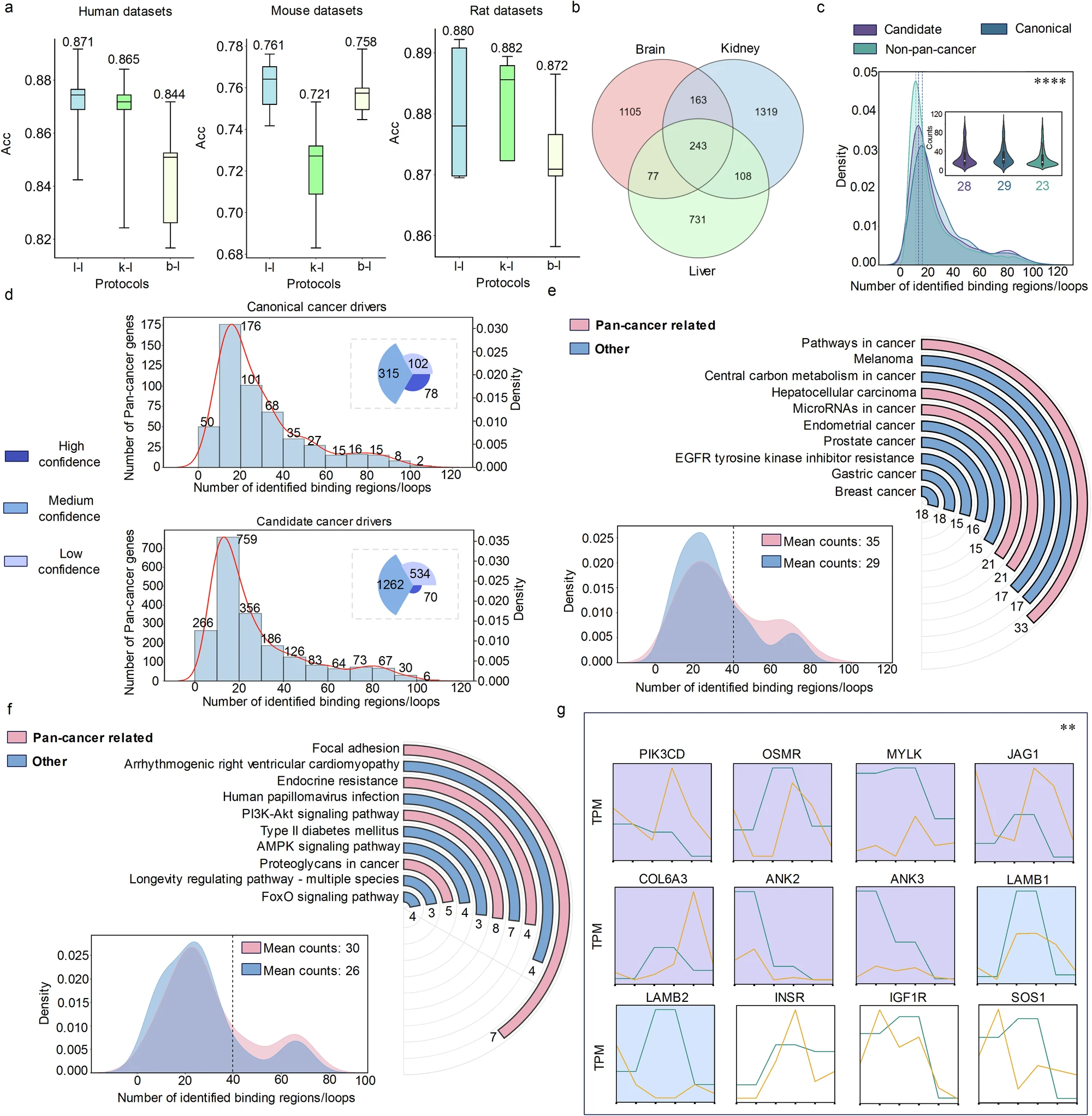
- Li, G., Su, X., Yang, Y. et al. Interpretability-guided RNA N 6 \text{N}^6 N6-methyladenosine modification site prediction with invertible neural networks. Commun Biol 8, 1022 (2025). https://doi.org/10.1038/s42003-025-08265-8
的 fig.5 中的 e、f 图:
复刻效果:
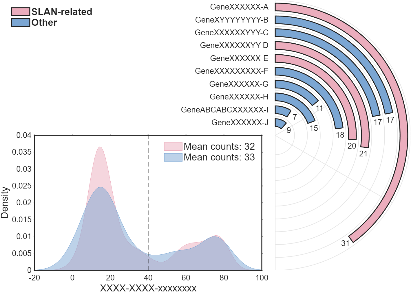

还是非常好看的:
正文
数据准备
这里展示一下每种数据大概长啥样:大家可以自行从excel、mat或者txt文件读取:
matlab
clc; clear
% 原图环形柱状图柱子长度显著性水平,顶部的数字表示富集基因的数量
% 这里我们直接随便编一下

Name = {'GeneXXXXXX-A', 'GeneXYYYYYYYY-B', 'GeneXXXXXXYYY-C', 'GeneXXXXXXYY-D', ...
        'GeneXXXXXX-E', 'GeneXXXXXXXXX-F', 'GeneXXXXXX-G', 'GeneXXXXXX-H', ...
        'GeneABCABCXXXXXX-I', 'GeneXXXXXX-J'};
Value = [31, 17, 17, 21, 20, 18, 11, 15, 7, 9];
Len = Value; % 我们这里直接长度和数字统一,可自行换成其他数值
Class = [1, 2, 2, 1, 1, 2, 2, 2, 2, 2];
ClassName = {'SLAN-related', 'Other'};

% 随机生成了一些 0-80 的数字,并随机将其分类(类1、类2)
rng(1)
Num = [randi([0, 80], [1, 50]), randi([10, 20], [1, 40]), randi([75, 80], [1, 10])];
NumClass = randi([1, 2], [1, 100]);


% 配色,这里只有两种颜色,如果类更多的话要增添更多颜色
CList = [235,173,189;
        123,166,211]./255;
原文中柱状图的柱子长度和标注的数值是不一样的,柱子长度代表显著性水平,顶部的数字表示富集基因的数量,我们弄一样或者不一样都可以。比如我们这段代码里面标注的数值和柱子长度就是对应的。变量 Class 和 NumClass 这里用来存储分类情况的数组,比如分了两类的话,其中的数值就只有1和2。
环形柱状图绘制
比较新的版本可以直接用极坐标区域相关函数绘制会非常方便,这里为了尽量照顾更多的版本,就硬画了网格线和柱子:
matlab
figure('Units','normalized', 'Position',[.1,.2,.7,.7]);
%% 环形柱状图
ax1 = axes('Parent',gcf, 'Position',[.05,.1,.9,.8], 'DataAspectRatio',[1,1,1], ...
    'XLim', [-2, 1], 'YLim', [-1,1], 'NextPlot','add', 'XColor','none', 'YColor','none');
N = length(Value); M = max(Len);
% 绘制环形柱状图网格
tt = linspace(pi/2, -pi/2, 100); xx = cos(tt); yy = sin(tt);
XX = repmat([xx.'; nan], [1, N]).*repmat(((1:N) + .5)./(N + .5), [101, 1]);
YY = repmat([yy.'; nan], [1, N]).*repmat(((1:N) + .5)./(N + .5), [101, 1]);
plot(XX(:), YY(:), 'LineWidth',1, 'Color',[1,1,1].*.9)
th = [pi/2, -pi/2, pi/6, -pi/6];
XX = [th.*0; cos(th); th.*nan];
YY = [th.*0; sin(th); th.*nan];
plot(XX(:), YY(:), 'LineWidth',1, 'Color',[1,1,1].*.9)
% 绘制柱状图
for i = 1:N
    R = (N - i + 1)./(N + .5); r = .3./(N + .5);
    TT = (tt - pi/2).*.8.*Len(i)./M + pi/2;
    XX = [cos(TT).*(R + r), cos(TT(end:-1:1)).*(R - r)];
    YY = [sin(TT).*(R + r), sin(TT(end:-1:1)).*(R - r)];
    fill(XX, YY, CList(Class(i),:), 'LineWidth',1.5)
    text(cos(TT(end)).*R + sin(TT(end))./(N)./2, sin(TT(end)).*R - cos(TT(end))./(N)./2, ...
        num2str(Value(i)), 'HorizontalAlignment','center', 'FontName','Arial', 'FontSize',13)
    text(-.05, R, Name{i}, 'HorizontalAlignment','right', 'FontName','Arial', 'FontSize',13)
end

for i = 1:max(Class)
    lgdHdl1(i) = fill([115,108,97,110,100], [97,114,101,114,32], CList(Class(i),:), 'LineWidth',1.5);
end
lgd1 = legend(lgdHdl1, ClassName, 'Box','off', 'FontName','Arial', ...
    'FontSize',16, 'FontWeight','bold', 'Location','northwest');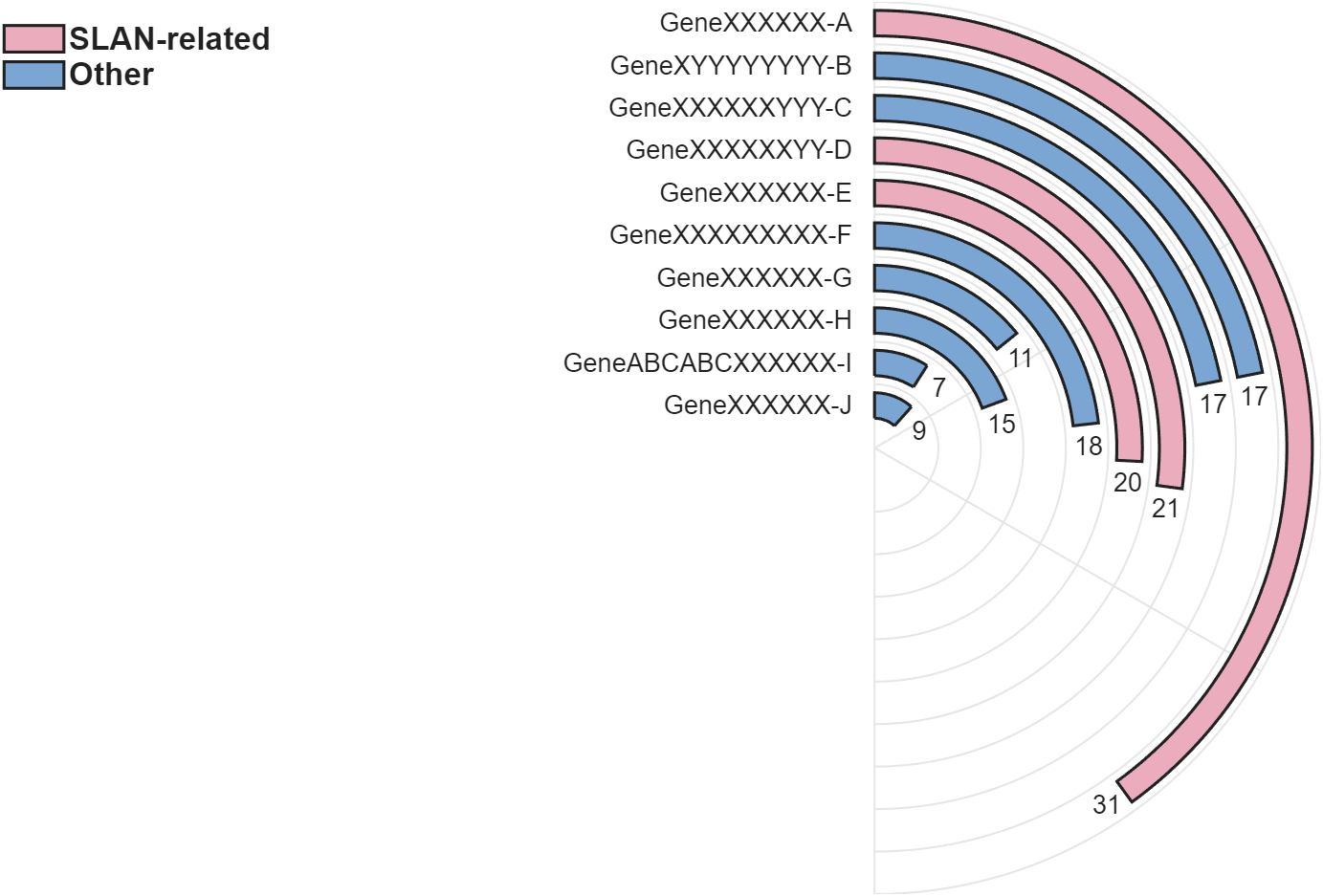
核密度图绘制
matlab
ax2 = axes('Parent',gcf, 'Position',[.18,.1,.42,.4], 'NextPlot','add', ...
    'XLim', [-20,100], 'LineWidth',1.5, 'Box','on', 'TickLength',[.001,0], ...
    'TickDir','out', 'FontSize',13);
xlabel(ax2, 'XXXX-XXXX-xxxxxxxx', 'FontName','Arial', 'FontSize',16)
ylabel(ax2, 'Density', 'FontName','Arial', 'FontSize',16)
xline(40, 'LineWidth',1, 'Alpha',1, 'LineStyle','--');

for i = 1:max(NumClass)
    x = Num(NumClass == i);
    [f, xi] = ksdensity(x);
    lgdHdl2(i) = area(xi, f, 'FaceColor',CList(i,:), 'EdgeColor',CList(i,:), 'FaceAlpha',.5);
    lgdtxt{i} = ['Mean counts: ' ,num2str(round(mean(x)))];
end
lgd2 = legend(lgdHdl2, ClassName, 'Box','off', 'FontName','Arial', ...
    'FontSize',16, 'Location','northeast');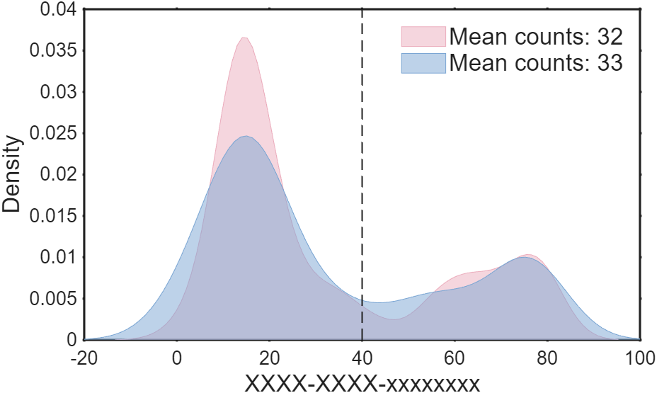
完整代码
完整代码(两类)
matlab
% 复刻自 | https://www.nature.com/articles/s42003-025-08265-8
% + Li, G., Su, X., Yang, Y. et al.
%   Interpretability-guided RNA N6-methyladenosine modification site prediction
%   with invertible neural networks. Commun Biol 8, 1022 (2025).
%   https://doi.org/10.1038/s42003-025-08265-8

clc; clear
% 原图环形柱状图柱子长度显著性水平,顶部的数字表示富集基因的数量
% 这里我们直接随便编一下

Name = {'GeneXXXXXX-A', 'GeneXYYYYYYYY-B', 'GeneXXXXXXYYY-C', 'GeneXXXXXXYY-D', ...
        'GeneXXXXXX-E', 'GeneXXXXXXXXX-F', 'GeneXXXXXX-G', 'GeneXXXXXX-H', ...
        'GeneABCABCXXXXXX-I', 'GeneXXXXXX-J'};
Value = [31, 17, 17, 21, 20, 18, 11, 15, 7, 9];
Len = Value; % 我们这里直接长度和数字统一,可自行换成其他数值
Class = [1, 2, 2, 1, 1, 2, 2, 2, 2, 2];
ClassName = {'SLAN-related', 'Other'};

% 随机生成了一些 0-80 的数字,并随机将其分类(类1、类2)
rng(1)
Num = [randi([0, 80], [1, 50]), randi([10, 20], [1, 40]), randi([75, 80], [1, 10])];
NumClass = randi([1, 2], [1, 100]);


% 配色,这里只有两种颜色,如果类更多的话要增添更多颜色
CList = [235,173,189;
        123,166,211]./255;


%% 开始绘图 ================================================================
figure('Units','normalized', 'Position',[.1,.2,.7,.7]);
%% 环形柱状图
ax1 = axes('Parent',gcf, 'Position',[.05,.1,.9,.8], 'DataAspectRatio',[1,1,1], ...
    'XLim', [-2, 1], 'YLim', [-1,1], 'NextPlot','add', 'XColor','none', 'YColor','none');
N = length(Value); M = max(Len);
% 绘制环形柱状图网格
tt = linspace(pi/2, -pi/2, 100); xx = cos(tt); yy = sin(tt);
XX = repmat([xx.'; nan], [1, N]).*repmat(((1:N) + .5)./(N + .5), [101, 1]);
YY = repmat([yy.'; nan], [1, N]).*repmat(((1:N) + .5)./(N + .5), [101, 1]);
plot(XX(:), YY(:), 'LineWidth',1, 'Color',[1,1,1].*.9)
th = [pi/2, -pi/2, pi/6, -pi/6];
XX = [th.*0; cos(th); th.*nan];
YY = [th.*0; sin(th); th.*nan];
plot(XX(:), YY(:), 'LineWidth',1, 'Color',[1,1,1].*.9)
% 绘制柱状图
for i = 1:N
    R = (N - i + 1)./(N + .5); r = .3./(N + .5);
    TT = (tt - pi/2).*.8.*Len(i)./M + pi/2;
    XX = [cos(TT).*(R + r), cos(TT(end:-1:1)).*(R - r)];
    YY = [sin(TT).*(R + r), sin(TT(end:-1:1)).*(R - r)];
    fill(XX, YY, CList(Class(i),:), 'LineWidth',1.5)
    text(cos(TT(end)).*R + sin(TT(end))./(N)./2, sin(TT(end)).*R - cos(TT(end))./(N)./2, ...
        num2str(Value(i)), 'HorizontalAlignment','center', 'FontName','Arial', 'FontSize',13)
    text(-.05, R, Name{i}, 'HorizontalAlignment','right', 'FontName','Arial', 'FontSize',13)
end

for i = 1:max(Class)
    lgdHdl1(i) = fill([115,108,97,110,100], [97,114,101,114,32], CList(Class(i),:), 'LineWidth',1.5);
end
lgd1 = legend(lgdHdl1, ClassName, 'Box','off', 'FontName','Arial', ...
    'FontSize',16, 'FontWeight','bold', 'Location','northwest');

%% 核密度图
ax2 = axes('Parent',gcf, 'Position',[.18,.1,.42,.4], 'NextPlot','add', ...
    'XLim', [-20,100], 'LineWidth',1.5, 'Box','on', 'TickLength',[.001,0], ...
    'TickDir','out', 'FontSize',13);
xlabel(ax2, 'XXXX-XXXX-xxxxxxxx', 'FontName','Arial', 'FontSize',16)
ylabel(ax2, 'Density', 'FontName','Arial', 'FontSize',16)
xline(40, 'LineWidth',1, 'Alpha',1, 'LineStyle','--');

for i = 1:max(NumClass)
    x = Num(NumClass == i);
    [f, xi] = ksdensity(x);
    lgdHdl2(i) = area(xi, f, 'FaceColor',CList(i,:), 'EdgeColor',CList(i,:), 'FaceAlpha',.5);
    lgdtxt{i} = ['Mean counts: ' ,num2str(round(mean(x)))];
end
lgd2 = legend(lgdHdl2, ClassName, 'Box','off', 'FontName','Arial', ...
    'FontSize',16, 'Location','northeast');
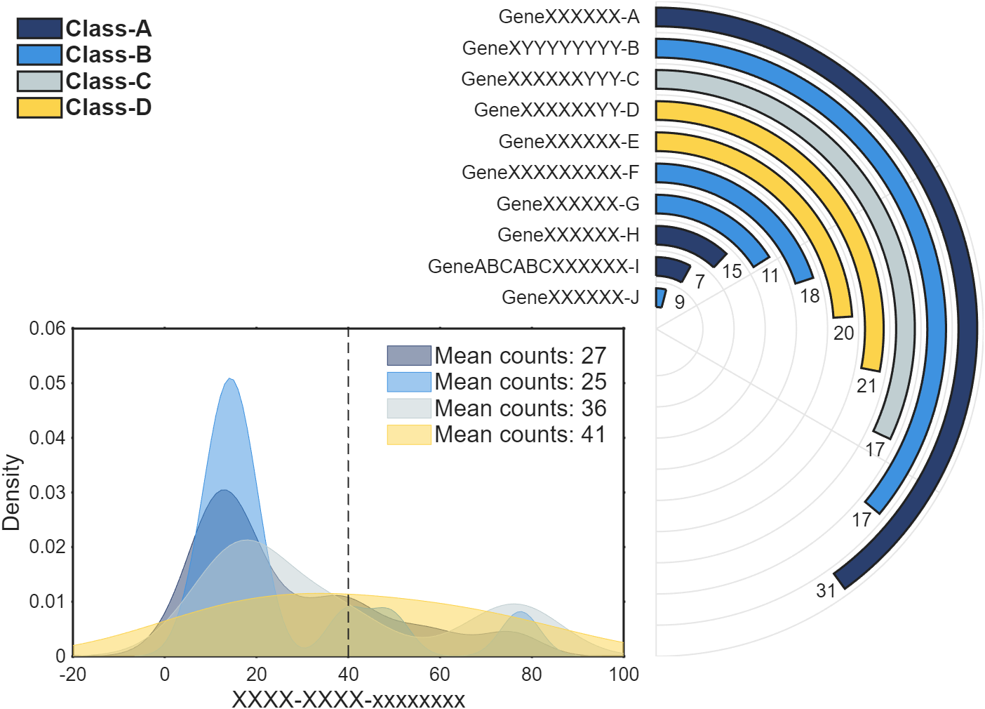
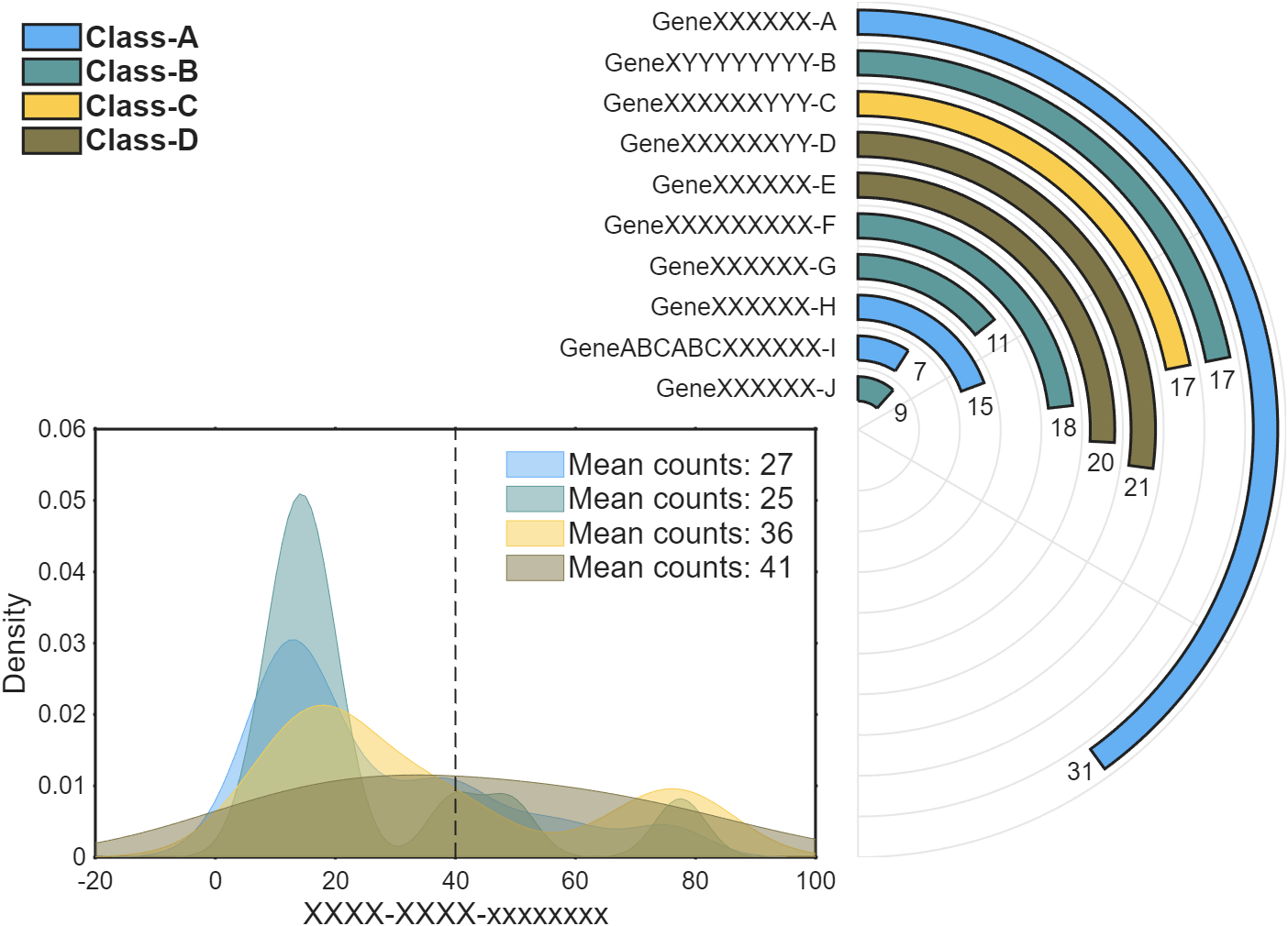
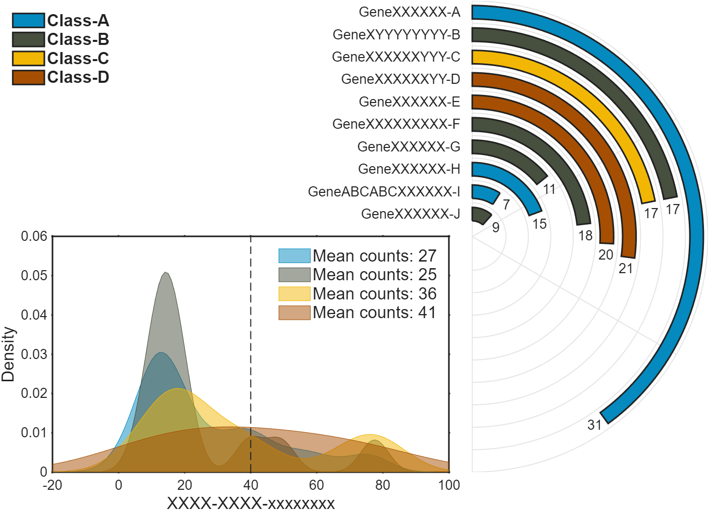
完整代码(更多类和更多配色)
写了一个例子,能更清晰展示怎么画分更多类的图:实际上有变动的只有前半部分。后面代码一模一样。
matlab
% 复刻自 | https://www.nature.com/articles/s42003-025-08265-8
% + Li, G., Su, X., Yang, Y. et al.
%   Interpretability-guided RNA N6-methyladenosine modification site prediction
%   with invertible neural networks. Commun Biol 8, 1022 (2025).
%   https://doi.org/10.1038/s42003-025-08265-8

clc; clear
% 原图环形柱状图柱子长度显著性水平,顶部的数字表示富集基因的数量
% 这里我们直接随便编一下

Name = {'GeneXXXXXX-A', 'GeneXYYYYYYYY-B', 'GeneXXXXXXYYY-C', 'GeneXXXXXXYY-D', ...
        'GeneXXXXXX-E', 'GeneXXXXXXXXX-F', 'GeneXXXXXX-G', 'GeneXXXXXX-H', ...
        'GeneABCABCXXXXXX-I', 'GeneXXXXXX-J'};
Value = [31, 17, 17, 21, 20, 18, 11, 15, 7, 9];
Len = 10:-1:1; % 我们这里直接长度和数字统一,可自行换成其他数值
Class = [1, 2, 3, 4, 4, 2, 2, 1, 1, 2];
ClassName = {'Class-A','Class-B','Class-C','Class-D'};

% 随机生成了一些 0-80 的数字,并随机将其分类(类1、类2、类3、类4)
rng(2)
Num = [randi([0, 80], [1, 50]), randi([10, 20], [1, 40]), randi([75, 80], [1, 10])];
NumClass = randi([1, 4], [1, 100]);

% 配色,如果类更多的话要增添更多颜色
CList = [0.3961    0.6863    0.9529
    0.3686    0.6039    0.6118
    0.9725    0.8039    0.3137
    0.5020    0.4706    0.2902];
% CList = [0.0157    0.5412    0.7490
%     0.2784    0.3098    0.2431
%     0.9490    0.7176    0.0196
%     0.6510    0.3098    0.0118
%     0.7490    0.1882    0.1882];
% CList = [0.0745    0.1922    0.4902
%     0.4941    0.6549    0.8275
%     0.5216    0.8275    0.7647
%     0.8510    0.5725    0.4745
%     0.9686    0.3176    0.0275];
% CList = [0.1647    0.2471    0.4314
%     0.2431    0.5725    0.8784
%     0.7529    0.8078    0.8196
%     0.9882    0.8275    0.2941
%     0.9686    0.5804    0.0353];


%% 开始绘图 ================================================================
figure('Units','normalized', 'Position',[.1,.2,.7,.7]);
%% 环形柱状图
ax1 = axes('Parent',gcf, 'Position',[.05,.1,.9,.8], 'DataAspectRatio',[1,1,1], ...
    'XLim', [-2, 1], 'YLim', [-1,1], 'NextPlot','add', 'XColor','none', 'YColor','none');
N = length(Value); M = max(Len);
% 绘制环形柱状图网格
tt = linspace(pi/2, -pi/2, 100); xx = cos(tt); yy = sin(tt);
XX = repmat([xx.'; nan], [1, N]).*repmat(((1:N) + .5)./(N + .5), [101, 1]);
YY = repmat([yy.'; nan], [1, N]).*repmat(((1:N) + .5)./(N + .5), [101, 1]);
plot(XX(:), YY(:), 'LineWidth',1, 'Color',[1,1,1].*.9)
th = [pi/2, -pi/2, pi/6, -pi/6];
XX = [th.*0; cos(th); th.*nan];
YY = [th.*0; sin(th); th.*nan];
plot(XX(:), YY(:), 'LineWidth',1, 'Color',[1,1,1].*.9)
% 绘制柱状图
for i = 1:N
    R = (N - i + 1)./(N + .5); r = .3./(N + .5);
    TT = (tt - pi/2).*.8.*Len(i)./M + pi/2;
    XX = [cos(TT).*(R + r), cos(TT(end:-1:1)).*(R - r)];
    YY = [sin(TT).*(R + r), sin(TT(end:-1:1)).*(R - r)];
    fill(XX, YY, CList(Class(i),:), 'LineWidth',1.5)
    text(cos(TT(end)).*R + sin(TT(end))./(N)./2, sin(TT(end)).*R - cos(TT(end))./(N)./2, ...
        num2str(Value(i)), 'HorizontalAlignment','center', 'FontName','Arial', 'FontSize',13)
    text(-.05, R, Name{i}, 'HorizontalAlignment','right', 'FontName','Arial', 'FontSize',13)
end
for i = 1:max(Class)
    lgdHdl1(i) = fill([115,108,97,110,100], [97,114,101,114,32], CList(Class(i),:), 'LineWidth',1.5);
end
lgd1 = legend(lgdHdl1, ClassName, 'Box','off', 'FontName','Arial', ...
    'FontSize',16, 'FontWeight','bold', 'Location','northwest');
%% 核密度图

ax2 = axes('Parent',gcf, 'Position',[.18,.1,.42,.4], 'NextPlot','add', ...
    'XLim', [-20,100], 'LineWidth',1.5, 'Box','on', 'TickLength',[.001,0], ...
    'TickDir','out', 'FontSize',13);
xlabel(ax2, 'XXXX-XXXX-xxxxxxxx', 'FontName','Arial', 'FontSize',16)
ylabel(ax2, 'Density', 'FontName','Arial', 'FontSize',16)
xline(40, 'LineWidth',1, 'Alpha',1, 'LineStyle','--');

for i = 1:max(NumClass)
    x = Num(NumClass == i);
    [f, xi] = ksdensity(x);
    lgdHdl2(i) = area(xi, f, 'FaceColor',CList(i,:), 'EdgeColor',CList(i,:), 'FaceAlpha',.5);
    lgdtxt{i} = ['Mean counts: ' ,num2str(round(mean(x)))];
end
lgd2 = legend(lgdHdl2, lgdtxt, 'Box','off', 'FontName','Arial', ...
    'FontSize',16, 'Location','northeast');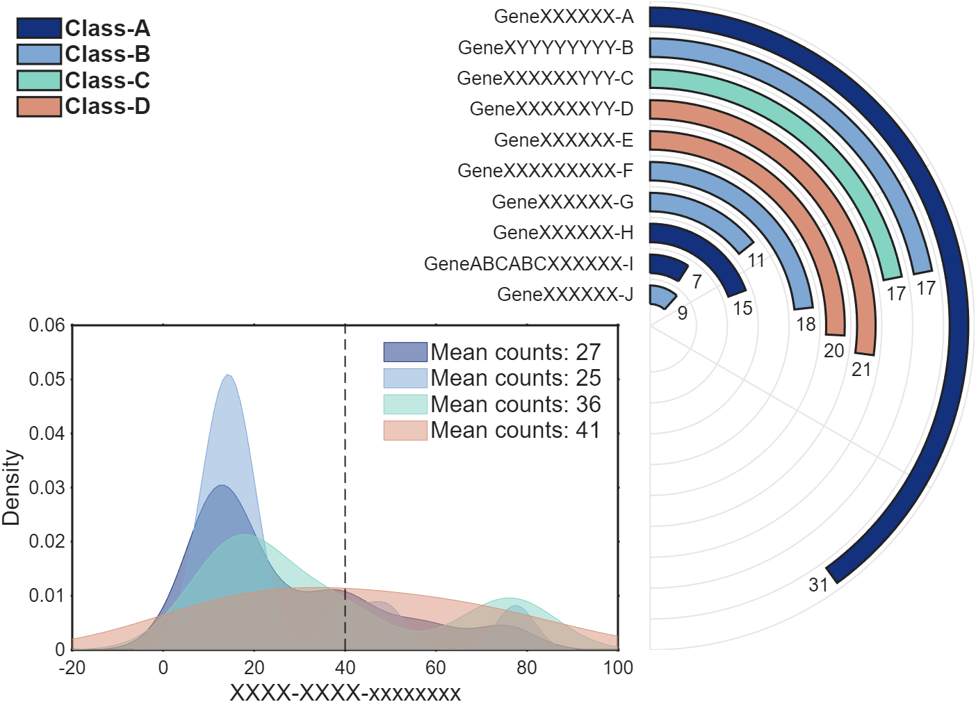

结
完整代码可以从以下gitee仓库获取: