MATLAB程序,用于三维点云的最小二乘拟合,支持平面、球面和二次曲面拟合,并提供可视化功能
Matlab
classdef PointCloudFitter
% 三维点云最小二乘拟合类
% 支持平面、球面、二次曲面拟合
properties
points; % 输入点云数据 (N×3矩阵)
fittedModel; % 拟合模型参数
residuals; % 残差
modelType; % 模型类型 ('plane', 'sphere', 'quadric')
fittingError; % 拟合误差
end
methods
function obj = PointCloudFitter(points)
% 构造函数
% 输入: points - N×3矩阵,每行表示一个点的[x,y,z]坐标
obj.points = points;
obj.modelType = '';
obj.fittedModel = [];
obj.residuals = [];
obj.fittingError = inf;
end
function obj = fitPlane(obj)
% 最小二乘平面拟合
% 平面方程: ax + by + cz + d = 0
% 输出: 更新obj.fittedModel = [a,b,c,d] (归一化法向量)
points = obj.points;
n = size(points, 1); % 点数
% 计算质心
centroid = mean(points, 1);
% 去中心化
centeredPoints = points - centroid;
% 计算协方差矩阵
covMat = (centeredPoints' * centeredPoints) / (n-1);
% 特征值分解
[V, D] = eig(covMat);
% 最小特征值对应的特征向量即为法向量
[~, idx] = min(diag(D));
normal = V(:, idx);
% 归一化法向量
normal = normal / norm(normal);
% 计算d: ax+by+cz+d=0 => d = -(a*x0+b*y0+c*z0)
a = normal(1);
b = normal(2);
c = normal(3);
d = -dot(normal, centroid);
% 存储模型参数
obj.fittedModel = [a, b, c, d];
obj.modelType = 'plane';
% 计算残差
distances = abs(a*points(:,1) + b*points(:,2) + c*points(:,3) + d) / sqrt(a^2 + b^2 + c^2);
obj.residuals = distances;
obj.fittingError = mean(distances.^2);
end
function obj = fitSphere(obj)
% 最小二乘球面拟合
% 球面方程: (x-a)^2 + (y-b)^2 + (z-c)^2 = r^2
% 输出: 更新obj.fittedModel = [a,b,c,r] (球心坐标和半径)
points = obj.points;
n = size(points, 1); % 点数
% 构建线性方程组
A = zeros(n, 4);
b = zeros(n, 1);
for i = 1:n
x = points(i, 1);
y = points(i, 2);
z = points(i, 3);
A(i, :) = [2*x, 2*y, 2*z, 1];
b(i) = x^2 + y^2 + z^2;
end
% 最小二乘求解
params = A \ b;
% 提取参数
a = params(1);
b = params(2);
c = params(3);
r_sq = params(4) + a^2 + b^2 + c^2;
% 计算半径
r = sqrt(r_sq);
% 存储模型参数
obj.fittedModel = [a, b, c, r];
obj.modelType = 'sphere';
% 计算残差
distances = sqrt((points(:,1)-a).^2 + (points(:,2)-b).^2 + (points(:,3)-c).^2) - r;
obj.residuals = distances;
obj.fittingError = mean(distances.^2);
end
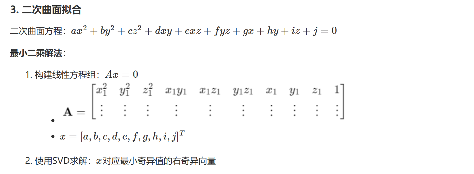
function obj = fitQuadricSurface(obj)
% 最小二乘二次曲面拟合
% 二次曲面方程: ax² + by² + cz² + dxy + exz + fyz + gx + hy + iz + j = 0
% 输出: 更新obj.fittedModel = [a,b,c,d,e,f,g,h,i,j]
points = obj.points;
n = size(points, 1); % 点数
% 构建线性方程组
A = zeros(n, 10);
for i = 1:n
x = points(i, 1);
y = points(i, 2);
z = points(i, 3);
A(i, :) = [x^2, y^2, z^2, x*y, x*z, y*z, x, y, z, 1];
end
% 使用SVD求解最小二乘问题
[~, ~, V] = svd(A);
params = V(:, end); % 最小奇异值对应的右奇异向量
% 存储模型参数
obj.fittedModel = params';
obj.modelType = 'quadric';
% 计算残差
a = params(1); b = params(2); c = params(3); d = params(4);
e = params(5); f = params(6); g = params(7); h = params(8);
i_val = params(9); j = params(10);
distances = a*points(:,1).^2 + b*points(:,2).^2 + c*points(:,3).^2 + ...
d*points(:,1).*points(:,2) + e*points(:,1).*points(:,3) + ...
f*points(:,2).*points(:,3) + g*points(:,1) + ...
h*points(:,2) + i_val*points(:,3) + j;
obj.residuals = distances;
obj.fittingError = mean(distances.^2);
end
function obj = fitBestModel(obj)
% 尝试多种模型并返回最佳拟合
models = {'plane', 'sphere', 'quadric'};
bestError = inf;
for i = 1:length(models)
switch models{i}
case 'plane'
tempObj = PointCloudFitter(obj.points);
tempObj = tempObj.fitPlane();
case 'sphere'
tempObj = PointCloudFitter(obj.points);
tempObj = tempObj.fitSphere();
case 'quadric'
tempObj = PointCloudFitter(obj.points);
tempObj = tempObj.fitQuadricSurface();
end
if tempObj.fittingError < bestError
bestError = tempObj.fittingError;
obj.fittedModel = tempObj.fittedModel;
obj.modelType = tempObj.modelType;
obj.residuals = tempObj.residuals;
obj.fittingError = tempObj.fittingError;
end
end
end
function visualize(obj)
% 可视化点云和拟合结果
figure('Name', '点云最小二乘拟合', 'NumberTitle', 'off');
hold on;
grid on;
axis equal;
view(3);
xlabel('X');
ylabel('Y');
zlabel('Z');
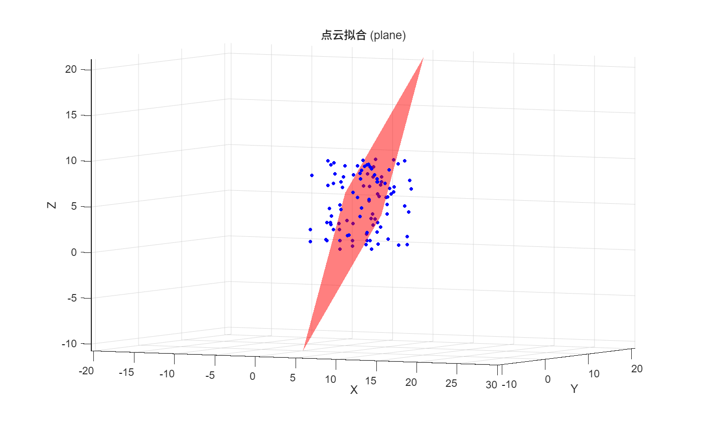
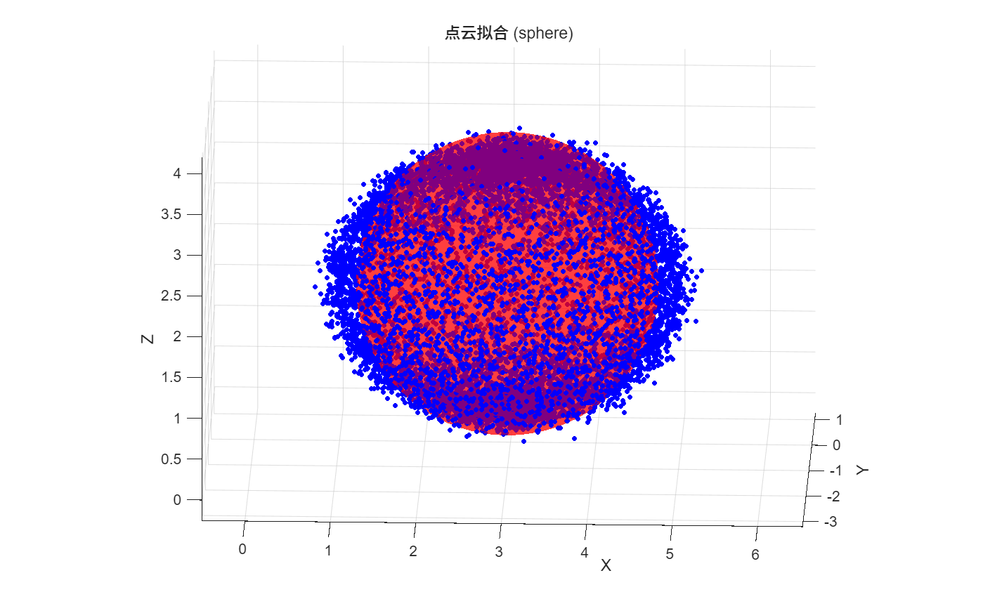
title(sprintf('点云拟合 (%s)', obj.modelType));
% 绘制原始点云
scatter3(obj.points(:,1), obj.points(:,2), obj.points(:,3), 10, 'b', 'filled');
% 绘制拟合结果
switch obj.modelType
case 'plane'
obj.visualizePlane();
case 'sphere'
obj.visualizeSphere();
case 'quadric'
obj.visualizeQuadric();
otherwise
error('未知模型类型');
end
% 绘制残差分布
figure('Name', '残差分布', 'NumberTitle', 'off');
histogram(obj.residuals, 50);
xlabel('残差');
ylabel('频数');
title(sprintf('%s拟合残差分布', obj.modelType));
grid on;
end
function visualizePlane(obj)
% 可视化拟合平面
params = obj.fittedModel;
a = params(1); b = params(2); c = params(3); d = params(4);
% 创建网格
[x, y] = meshgrid(linspace(min(obj.points(:,1)), max(obj.points(:,1)), 10), ...
linspace(min(obj.points(:,2)), max(obj.points(:,2)), 10));
% 计算z值 (如果c ≠ 0)
if abs(c) > 1e-6
z = (-a*x - b*y - d) / c;
surf(x, y, z, 'FaceAlpha', 0.5, 'EdgeColor', 'none', 'FaceColor', 'r');
elseif abs(a) > 1e-6 % 平面平行于z轴
z = linspace(min(obj.points(:,3)), max(obj.points(:,3)), 10);
y = (-a*x - c*z - d) / b;
surf(x, y, reshape(repmat(z, 10, 1), 10, 10), 'FaceAlpha', 0.5, 'EdgeColor', 'none', 'FaceColor', 'r');
else % 平面平行于y轴
z = linspace(min(obj.points(:,3)), max(obj.points(:,3)), 10);
x_grid = (-b*y - c*z - d) / a;
surf(reshape(repmat(x_grid, 10, 1), 10, 10), y, z, 'FaceAlpha', 0.5, 'EdgeColor', 'none', 'FaceColor', 'r');
end
end
function visualizeSphere(obj)
% 可视化拟合球面
params = obj.fittedModel;
center = params(1:3);
radius = params(4);
% 创建球面网格
[x, y, z] = sphere(50);
x = x * radius + center(1);
y = y * radius + center(2);
z = z * radius + center(3);
% 绘制球面
surf(x, y, z, 'FaceAlpha', 0.5, 'EdgeColor', 'none', 'FaceColor', 'r');
end
function visualizeQuadric(obj)
% 可视化二次曲面(简化为椭球)
params = obj.fittedModel;
a = params(1); b = params(2); c = params(3); d = params(4);
e = params(5); f = params(6); g = params(7); h = params(8);
i_val = params(9); j = params(10);
% 简化处理:假设为椭球
figure;
fimplicit3(@(x,y,z) a*x.^2 + b*y.^2 + c*z.^2 + d*x.*y + e*x.*z + f*y.*z + ...
g*x + h*y + i_val*z + j, ...
[-1 1 -1 1 -1 1]*max(max(abs(obj.points))));
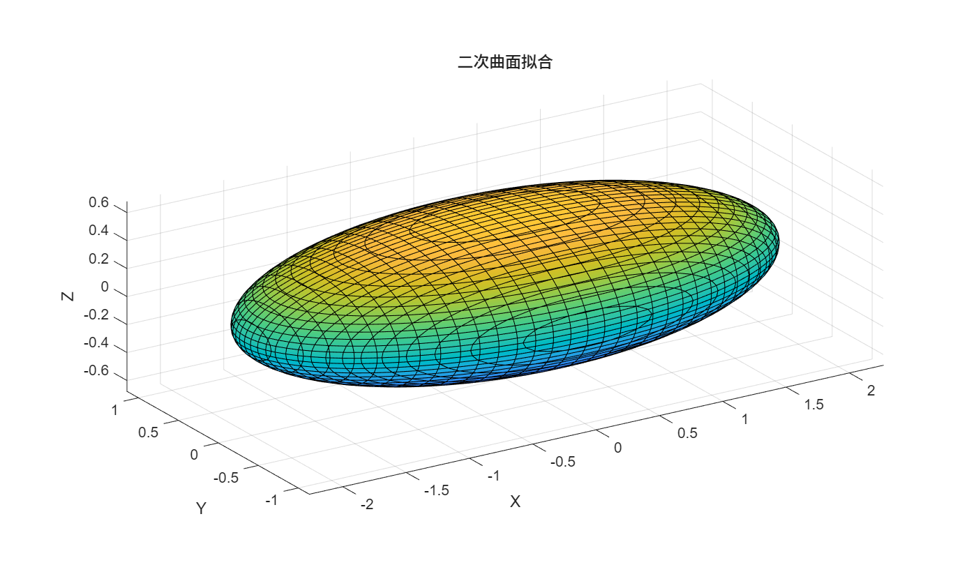
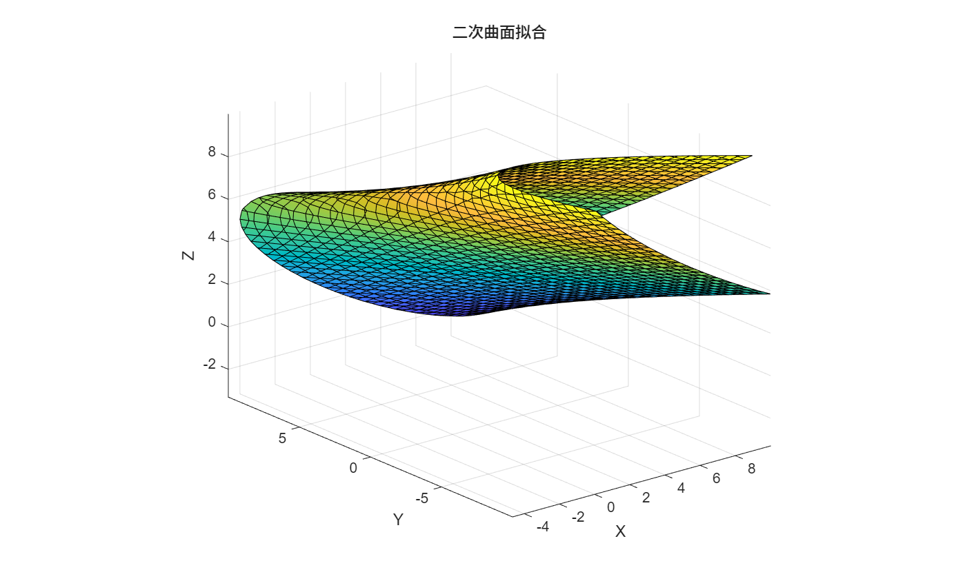
title('二次曲面拟合');
xlabel('X'); ylabel('Y'); zlabel('Z');
grid on;
axis equal;
end
function report(obj)
% 输出拟合报告
fprintf('\n===== 点云拟合报告 =====\n');
fprintf('模型类型: %s\n', obj.modelType);
fprintf('拟合误差(RMSE): %.6f\n', sqrt(obj.fittingError));
fprintf('最大残差: %.6f\n', max(abs(obj.residuals)));
fprintf('最小残差: %.6f\n', min(abs(obj.residuals)));
fprintf('平均残差: %.6f\n', mean(abs(obj.residuals)));
fprintf('残差标准差: %.6f\n', std(obj.residuals));
switch obj.modelType
case 'plane'
fprintf('\n平面参数: ax + by + cz + d = 0\n');
fprintf('a = %.6f, b = %.6f, c = %.6f, d = %.6f\n', obj.fittedModel);
fprintf('法向量: [%.6f, %.6f, %.6f]\n', obj.fittedModel(1:3));
case 'sphere'
fprintf('\n球面参数: (x-a)^2 + (y-b)^2 + (z-c)^2 = r^2\n');
fprintf('球心: (%.6f, %.6f, %.6f)\n', obj.fittedModel(1:3));
fprintf('半径: %.6f\n', obj.fittedModel(4));
case 'quadric'
fprintf('\n二次曲面参数: ax² + by² + cz² + dxy + exz + fyz + gx + hy + iz + j = 0\n');
labels = {'a', 'b', 'c', 'd', 'e', 'f', 'g', 'h', 'i', 'j'};
for k = 1:10
fprintf('%s = %.6f\n', labels{k}, obj.fittedModel(k));
end
end
fprintf('========================\n');
end
function runDemo()
% 运行演示
fprintf('三维点云最小二乘拟合演示\n');
% 生成示例点云
fprintf('生成示例点云...\n');
% 平面点云
[x, y] = meshgrid(linspace(-1, 1, 50), linspace(-1, 1, 50));
z = 0.5*x + 0.3*y + 0.2 + 0.05*randn(size(x));
planePoints = [x(:), y(:), z(:)];
% 球面点云
[x_s, y_s, z_s] = sphere(50);
spherePoints = [x_s(:)*0.8+0.5, y_s(:)*0.8+0.5, z_s(:)*0.8+0.5];
spherePoints = spherePoints + 0.02*randn(size(spherePoints));
% 椭球点云
[x_e, y_e, z_e] = ellipsoid(0, 0, 0, 1, 0.7, 0.5, 50);
ellipsoidPoints = [x_e(:), y_e(:), z_e(:)];
ellipsoidPoints = ellipsoidPoints + 0.03*randn(size(ellipsoidPoints));
% 平面拟合演示
fprintf('\n=== 平面拟合演示 ===\n');
planeFitter = PointCloudFitter(planePoints);
planeFitter = planeFitter.fitPlane();
planeFitter.visualize();
planeFitter.report();
% 球面拟合演示
fprintf('\n=== 球面拟合演示 ===\n');
sphereFitter = PointCloudFitter(spherePoints);
sphereFitter = sphereFitter.fitSphere();
sphereFitter.visualize();
sphereFitter.report();
% 二次曲面拟合演示
fprintf('\n=== 二次曲面拟合演示 ===\n');
quadricFitter = PointCloudFitter(ellipsoidPoints);
quadricFitter = quadricFitter.fitQuadricSurface();
quadricFitter.visualize();
quadricFitter.report();
% 自动选择最佳模型
fprintf('\n=== 自动选择最佳模型演示 ===\n');
% 添加一些噪声点
noisyPoints = [planePoints; 0.5*randn(20,3)];
autoFitter = PointCloudFitter(noisyPoints);
autoFitter = autoFitter.fitBestModel();
autoFitter.visualize();
autoFitter.report();
end
end
end测试代码:
Matlab
clc;clear all;close all;
flag=4;

if flag==1%平面

    % 生成随机点云
    points = rand(100, 3) * 10;

    % 创建拟合器
    fitter = PointCloudFitter(points);

    % 拟合平面
    fitter = fitter.fitPlane();

    % 可视化结果
    fitter.visualize();

    % 输出报告
    fitter.report();

elseif flag==2%球面
    % 生成球面点云
    [x, y, z] = sphere(100);
    points = [x(:)*2+3, y(:)*2-1, z(:)*1.5+2] + 0.1*randn(101^2, 3);

    % 创建拟合器
    fitter = PointCloudFitter(points);

    % 拟合球面
    fitter = fitter.fitSphere();

    % 可视化结果
    fitter.visualize();

    % 输出报告
    fitter.report();

elseif flag==3

    % 生成椭球点云
    [x, y, z] = ellipsoid(0, 0, 0, 2, 1, 0.5, 100);
    points = [x(:), y(:), z(:)] + 0.1*randn(101^2, 3);

    % 创建拟合器
    fitter = PointCloudFitter(points);

    % 拟合二次曲面
    fitter = fitter.fitQuadricSurface();

    % 可视化结果
    fitter.visualize();

    % 输出报告
    fitter.report();
else%自动选择最佳模型
    % 生成混合点云
    planePoints = [rand(100,2)*10, 0.5*rand(100,1)*10];
    spherePoints = [randn(100,3)*0.5 + [5,5,5]];
    points = [planePoints; spherePoints];

    % 创建拟合器
    fitter = PointCloudFitter(points);

    % 自动选择最佳模型
    fitter = fitter.fitBestModel();

    % 可视化结果
    fitter.visualize();

    % 输出报告
    fitter.report();

end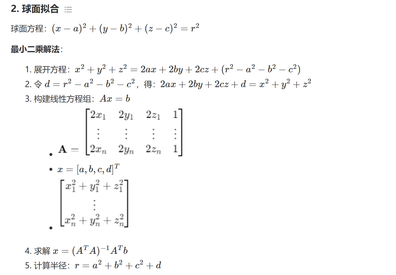
扩展功能
1. 鲁棒拟合(RANSAC)
Matlab
function obj = robustFitPlane(obj, maxIterations, distanceThreshold)
    % 使用RANSAC进行鲁棒平面拟合
    % 输入:
    %   maxIterations - 最大迭代次数
    %   distanceThreshold - 距离阈值

    bestInliers = [];
    bestModel = [];
    bestError = inf;
    n = size(obj.points, 1);

    for iter = 1:maxIterations
        % 随机选择3个点
        sampleIdx = randperm(n, 3);
        samplePts = obj.points(sampleIdx, :);

        % 拟合平面
        tempFitter = PointCloudFitter(samplePts);
        tempFitter = tempFitter.fitPlane();
        model = tempFitter.fittedModel;

        % 计算所有点到平面的距离
        a = model(1); b = model(2); c = model(3); d = model(4);
        distances = abs(a*obj.points(:,1) + b*obj.points(:,2) + c*obj.points(:,3) + d) / sqrt(a^2 + b^2 + c^2);

        % 统计内点
        inliers = find(distances < distanceThreshold);
        numInliers = length(inliers);

        % 更新最佳模型
        if numInliers > bestInliers
            bestInliers = inliers;
            bestModel = model;
            bestError = mean(distances(inliers).^2);
        end
    end

    % 使用所有内点重新拟合
    if ~isempty(bestInliers)
        inlierPts = obj.points(bestInliers, :);
        finalFitter = PointCloudFitter(inlierPts);
        finalFitter = finalFitter.fitPlane();
        obj.fittedModel = finalFitter.fittedModel;
        obj.modelType = 'plane';
        obj.residuals = finalFitter.residuals;
        obj.fittingError = finalFitter.fittingError;
    else
        obj.fittedModel = bestModel;
        obj.modelType = 'plane';
        obj.residuals = distances;
        obj.fittingError = bestError;
    end
end
2. 加权最小二乘
Matlab
function obj = weightedFitPlane(obj, weights)
    % 加权最小二乘平面拟合
    % 输入: weights - 权重向量 (N×1)

    points = obj.points;
    n = size(points, 1);

    % 计算加权质心
    centroid = sum(bsxfun(@times, points, weights), 1) / sum(weights);

    % 去中心化
    centeredPoints = bsxfun(@minus, points, centroid);

    % 构建加权协方差矩阵
    W = diag(weights);
    covMat = centeredPoints' * W * centeredPoints / (sum(weights) - 1);

    % 特征值分解
    [V, D] = eig(covMat);

    % 最小特征值对应的特征向量即为法向量
    [~, idx] = min(diag(D));
    normal = V(:, idx);

    % 归一化法向量
    normal = normal / norm(normal);

    % 计算d
    a = normal(1); b = normal(2); c = normal(3);
    d = -dot(normal, centroid);

    % 存储模型参数
    obj.fittedModel = [a, b, c, d];
    obj.modelType = 'plane';

    % 计算残差
    distances = abs(a*points(:,1) + b*points(:,2) + c*points(:,3) + d) / sqrt(a^2 + b^2 + c^2);
    obj.residuals = distances;
    obj.fittingError = mean(weights .* distances.^2);
end- 点云法线估计
Matlab
function normals = estimateNormals(obj, k)
    % 估计点云法线
    % 输入: k - 近邻点数
    % 输出: normals - 法线向量 (N×3)

    n = size(obj.points, 1);
    normals = zeros(n, 3);

    for i = 1:n
        % 计算当前点到所有点的距离
        dists = sum((obj.points - obj.points(i, :)).^2, 2);

        % 找到k个最近邻
        [~, idx] = mink(dists, k+1); % 包括自身
        idx = idx(2:end); % 排除自身

        % 使用近邻点拟合平面
        neighborPts = obj.points(idx, :);
        tempFitter = PointCloudFitter(neighborPts);
        tempFitter = tempFitter.fitPlane();

        % 获取法线
        normal = tempFitter.fittedModel(1:3);
        normals(i, :) = normal;
    end

    % 统一法线方向
    refVector = mean(obj.points, 1) - obj.points;
    dotProducts = sum(bsxfun(@times, normals, refVector), 2);
    flipIdx = dotProducts < 0;
    normals(flipIdx, :) = -normals(flipIdx, :);
end
结果: