注:本文为 "浮点运算" 相关译文,机翻未校。
略作重排,如有内容异常,请看原文。
csdn 篇幅所限,多篇连载。
An Error Analysis Example: The Quadratic Formula / 误差分析示例:二次方程求根公式
An interesting example of error analysis using formulas (19), (20) and (21) occurs in the quadratic formula −b±b2−4ac2a\frac{{ - b \pm \sqrt {{b^2} - 4ac} }}{{2a}}2a−b±b2−4ac .
利用公式 (19)、(20) 和 (21) 进行误差分析的一个有趣例子出现在二次方程求根公式 −b±b2−4ac2a\frac{{ - b \pm \sqrt {{b^2} - 4ac} }}{{2a}}2a−b±b2−4ac 中。
"Cancellation" on page 179, explained how rewriting the equation will eliminate the potential cancellation caused by the ± operation. But there is another potential cancellation that can occur when computing d=b2−4acd = b^2 - 4acd=b2−4ac. This one cannot be eliminated by a simple rearrangement of the formula. Roughly speaking, when b2≈4acb^2 \approx 4acb2≈4ac, rounding error can contaminate up to half the digits in the roots computed with the quadratic formula. Here is an informal proof (another approach to estimating the error in the quadratic formula appears in Kahan 1972).
本文 "相消误差" 小节中,阐述了如何通过改写方程来消除由 ±\pm± 运算引发的潜在相消误差。但在计算 d=b2−4acd = b^2 - 4acd=b2−4ac 时,还会出现另一种潜在的相消误差,这种误差无法通过简单的公式重新整理来消除。粗略来说,当 b2≈4acb^2 \approx 4acb2≈4ac 时,舍入误差可能会污染由二次方程求根公式计算出的根中多达一半的有效数字。以下是一个非形式化的证明(卡汉在 1972 年的文献中提出了另一种估算二次方程求根公式误差的方法)。
If b2≈4acb^2 \approx4acb2≈4ac, rounding error can contaminate up to half the digits in the roots computed with the quadratic formula −b±b2−4ac2a\frac{{ - b \pm \sqrt {{b^2} - 4ac} }}{{2a}}2a−b±b2−4ac .
若 b2≈4acb^2 \approx 4acb2≈4ac,舍入误差可能会污染由二次方程求根公式 −b±b2−4ac2a\frac{{ - b \pm \sqrt {{b^2} - 4ac} }}{{2a}}2a−b±b2−4ac 计算出的根中多达一半的有效数字。
Proof: Write (b⊗b)⊖(4a⊗c)=(b2(1+δ1)−4ac(1+δ2))(1+δ3)(b \otimes b) \ominus (4a \otimes c) = (b^2(1+\delta_1) - 4ac(1+\delta_2))(1+\delta_3)(b⊗b)⊖(4a⊗c)=(b2(1+δ1)−4ac(1+δ2))(1+δ3), where ∣δi∣≤ε|\delta_i| \leq \varepsilon∣δi∣≤ε. Using d=b2−4acd = b^2 - 4acd=b2−4ac, this can be rewritten as (d(1+δ1)−4ac(δ2−δ1))(1+δ3)(d(1+\delta_1) - 4ac(\delta_2-\delta_1))(1+\delta_3)(d(1+δ1)−4ac(δ2−δ1))(1+δ3). To get an estimate for the size of this error, ignore second order terms in δi\delta_iδi, in which case the absolute error is d(δ1+δ3)−4acδ4d(\delta_1+\delta_3) - 4ac\delta_4d(δ1+δ3)−4acδ4, where ∣δ4∣=∣δ1−δ2∣≤2ε|\delta_4| = |\delta_1-\delta_2| \leq 2\varepsilon∣δ4∣=∣δ1−δ2∣≤2ε.
Since d≪4acd \ll 4acd≪4ac, the first term d(δ1+δ3)d(\delta_1+\delta_3)d(δ1+δ3) can be ignored. To estimate the second term, use the fact that ax2+bx+c=a(x−r1)(x−r2)ax^2+bx+c = a(x-r_1)(x-r_2)ax2+bx+c=a(x−r1)(x−r2), so ar1r2=car_1r_2 = car1r2=c. Since
b2≈4acb^2 \approx 4acb2≈4ac, then r1≈r2r_1 \approx r_2r1≈r2, so the second error term is 4acδ4=4a2r12δ44ac\delta_4 = 4a^2r_1^2\delta_44acδ4=4a2r12δ4. Thus the computed value of d\sqrt{d}d is d+4a2r12δ4\sqrt{d + 4a^2r_1^2\delta_4}d+4a2r12δ4 . The inequality p−q≤p2−q2≤p2+q2≤p+qp-q \leq \sqrt{p^2-q^2} \leq \sqrt{p^2+q^2} \leq p+qp−q≤p2−q2 ≤p2+q2 ≤p+q (p≥q>0p \geq q > 0p≥q>0)
shows that d+4a2r12δ4=d+E\sqrt{d + 4a^2r_1^2\delta_4} = \sqrt{d} + Ed+4a2r12δ4 =d +E, where ∣E∣≤4a2r12∣δ4∣=2∣a∣r1∣δ4∣|E| \leq \sqrt{4a^2r_1^2|\delta_4|} = 2|a|r_1\sqrt{|\delta_4|}∣E∣≤4a2r12∣δ4∣ =2∣a∣r1∣δ4∣ , so the absolute error in d/(2a)\sqrt{d}/(2a)d /(2a) is about r1∣δ4∣r_1\sqrt{|\delta_4|}r1∣δ4∣ . Since ∣δ4∣≈β−p|\delta_4| \approx \beta^{-p}∣δ4∣≈β−p, ∣δ4∣≈β−p/2\sqrt{|\delta_4|} \approx \beta^{-p/2}∣δ4∣ ≈β−p/2, and thus the absolute error of r1∣δ4∣r_1\sqrt{|\delta_4|}r1∣δ4∣ destroys the bottom half of the bits of the roots r1≈r2r_1 \approx r_2r1≈r2. In other words, since the calculation of the roots involves computing with d/(2a)\sqrt{d}/(2a)d /(2a), and this expression does not have meaningful bits in the position corresponding to the lower order half of rir_iri, then the lower order bits of rir_iri cannot be meaningful. ∎
证明:
将 (b⊗b)⊖(4a⊗c)(b \otimes b) \ominus (4a \otimes c)(b⊗b)⊖(4a⊗c) 写成 (b⊗b)⊖(4a⊗c)=(b2(1+δ1)−4ac(1+δ2))(1+δ3),(b \otimes b) \ominus (4a \otimes c) = \bigl(b^2(1+\delta_1) - 4ac(1+\delta_2)\bigr)(1+\delta_3),(b⊗b)⊖(4a⊗c)=(b2(1+δ1)−4ac(1+δ2))(1+δ3), 其中 ∣δi∣≤ε|\delta_i| \leq \varepsilon∣δi∣≤ε。
令 d=b2−4acd = b^2 - 4acd=b2−4ac,上式可改写为 (d(1+δ1)−4ac(δ2−δ1))(1+δ3).\bigl(d(1+\delta_1) - 4ac(\delta_2-\delta_1)\bigr)(1+\delta_3).(d(1+δ1)−4ac(δ2−δ1))(1+δ3). 为估计该误差的大小,忽略 δi\delta_iδi 的二阶项,此时绝对误差为 d(δ1+δ3)−4acδ4,d(\delta_1+\delta_3) - 4ac\delta_4,d(δ1+δ3)−4acδ4, 其中 ∣δ4∣=∣δ1−δ2∣≤2ε|\delta_4| = |\delta_1-\delta_2| \leq 2\varepsilon∣δ4∣=∣δ1−δ2∣≤2ε。由于 d≪4acd \ll 4acd≪4ac,第一项 d(δ1+δ3)d(\delta_1+\delta_3)d(δ1+δ3) 可忽略。为估计第二项,利用 ax2+bx+c=a(x−r1)(x−r2)ax^2+bx+c = a(x-r_1)(x-r_2)ax2+bx+c=a(x−r1)(x−r2),于是有 ar1r2=car_1r_2 = car1r2=c。由 b2≈4acb^2 \approx 4acb2≈4ac 可知 r1≈r2r_1 \approx r_2r1≈r2,因此第二个误差项为 4acδ4=4a2r12δ4.4ac\delta_4 = 4a^2r_1^2\delta_4.4acδ4=4a2r12δ4. 从而 d\sqrt{d}d 的计算值为 d+4a2r12δ4.\sqrt{d + 4a^2r_1^2\delta_4}.d+4a2r12δ4 . 不等式 p−q≤p2−q2≤p2+q2≤p+q(p≥q>0)p-q \leq \sqrt{p^2-q^2} \leq \sqrt{p^2+q^2} \leq p+q \quad (p \geq q > 0)p−q≤p2−q2 ≤p2+q2 ≤p+q(p≥q>0)
可得 d+E≤d+E\sqrt {d + E} \leq \sqrt {d}+\sqrt {E}d+E ≤d +E (其中 E=4a2r12δ4E=4a^2r_1^2\delta_4E=4a2r12δ4),因此 d\sqrt {d}d 的绝对误差约为 E=2ar1∣δ4∣\sqrt {E}=2ar_1\sqrt {|\delta_4|}E =2ar1∣δ4∣ 。由于 ∣δ4∣≈β−p|\delta_4| \approx \beta^{-p}∣δ4∣≈β−p,则 ∣δ4∣≈β−p/2\sqrt {|\delta_4|}\approx\beta^{-p/2}∣δ4∣ ≈β−p/2,进而 d/(2a)\sqrt {d}/(2a)d /(2a) 的绝对误差会破坏根 r1≈r2r_1 \approx r_2r1≈r2 的低半部分二进制位。换言之,因为根的计算涉及对 d/(2a)\sqrt {d}/(2a)d /(2a) 的运算,而该表达式在对应 rir_iri 低半阶位的位置上不存在有效位,所以 rir_iri 的低阶位也无有效意义。❚
- In this informal proof, assume that β=2\beta = 2β=2 so that multiplication by 4 is exact and doesn't require a δi\delta_iδi.
在本非形式化证明中,假定基数 β=2\beta = 2β=2,因此乘以 4 的运算为精确运算,无需引入误差项 δi\delta_iδi。*
Finally, we turn to the proof of Theorem 6. It is based on the following fact, which is proven in "Theorem 14 and Theorem 8" on page 243.
最后,我们来证明定理 6,该证明基于本文 "定理 14 与定理 8" 小节中已证明的一个结论。
Theorem 14
定理 14
Let 0<k<p0<k<p0<k<p , and set m=βk+1m=\beta^{k}+1m=βk+1 , and assume that floating-point operations are exactly rounded. Then ((m⊗x)⊖(m⊗x⊖x))((m \otimes x) \ominus (m \otimes x \ominus x))((m⊗x)⊖(m⊗x⊖x)) is exactly equal to xxx rounded to p−kp-kp−k significant digits. More precisely, xxx is rounded by taking the significand of xxx, imagining a radix point just left of the kkk least significant digits and rounding to an integer.
设 0<k<p0<k<p0<k<p,令 m=βk+1m=\beta^{k}+1m=βk+1,且假设浮点运算为精确舍入。则运算式 ((m⊗x)⊖(m⊗x⊖x))((m \otimes x) \ominus (m \otimes x \ominus x))((m⊗x)⊖(m⊗x⊖x)) 的结果恰好等于将 xxx 舍入至 p−kp-kp−k 位有效数字后的值。更具体地说,对 xxx 的舍入操作过程为:取 xxx 的尾数,在其最后 kkk 位有效数字左侧虚拟一个小数点,再将其舍入为整数。
Proof of Theorem 6
定理 6 的证明
By Theorem 14, xhx_{h}xh is xxx rounded to p−k=⌊p/2⌋p-k=\lfloor p / 2\rfloorp−k=⌊p/2⌋ places. If there is no carry out, then certainly xhx_{h}xh can be represented with ⌊p/2⌋\lfloor p / 2\rfloor⌊p/2⌋ significant digits. Suppose there is a carry-out. If x=x0.x1...xp−1×βex=x_0.x_1...x_{p-1} \times\beta^{e}x=x0.x1...xp−1×βe , then rounding adds 1 to xp−k−1x_{p-k-1}xp−k−1 , and the only way there can be a carry-out is if xp−k−1=β−1x_{p-k-1}=\beta-1xp−k−1=β−1 , but then the low order digit of xhx_{h}xh is 1+xp−k−1=01+x_{p-k-1}=01+xp−k−1=0 , and so again xhx_{h}xh is representable in ⌊p/2⌋\lfloor p / 2\rfloor⌊p/2⌋ digits.
由定理 14 可知,xhx_hxh 是将 xxx 舍入至 p−k=⌊p/2⌋p-k=\lfloor p / 2\rfloorp−k=⌊p/2⌋ 位有效数字后的值。若舍入过程中无进位产生,xhx_hxh 显然可由 ⌊p/2⌋\lfloor p / 2\rfloor⌊p/2⌋ 位有效数字表示。假设舍入时出现进位,设 xxx 的浮点表示为 x=x0.x1...xp−1×βex=x_0.x_1...x_{p-1} \times\beta^{e}x=x0.x1...xp−1×βe,舍入操作会给 xp−k−1x_{p-k-1}xp−k−1 位加 1,而产生进位的唯一情况是 xp−k−1=β−1x_{p-k-1}=\beta-1xp−k−1=β−1,此时 xhx_hxh 的最低阶位为 1+xp−k−1=01+x_{p-k-1}=01+xp−k−1=0,因此 xhx_hxh 仍可由 ⌊p/2⌋\lfloor p / 2\rfloor⌊p/2⌋ 位有效数字表示。
To deal with xlx_{l}xl , scale xxx to be an integer satisfying βp−1≤x≤βp−1\beta^{p-1} ≤x ≤\beta^{p}-1βp−1≤x≤βp−1 .Let x=xˉh+xˉlx=\bar {x}{h}+\bar {x}{l}x=xˉh+xˉl where xˉh\bar {x}{h}xˉh is the p−kp-kp−k high order digits of xxx, and xˉl\bar {x}{l}xˉl is the kkk low order digits. There are three cases to consider. If xˉl<(β/2)βk−1\bar {x}{l}<(\beta / 2) \beta^{k-1}xˉl<(β/2)βk−1 ,then rounding xxx to p−kp-kp−k places is the same as chopping and xh=xˉhx{h}=\bar {x}{h}xh=xˉh , and xl=xˉlx{l}=\bar {x}{l}xl=xˉl .Since xˉl\bar {x}{l}xˉl has at most kkk digits, if ppp is even, then xˉl\bar {x}{l}xˉl has at most k=⌈p/2⌉=⌊p/2⌋k= \lceil p / 2\rceil=\lfloor p / 2\rfloork=⌈p/2⌉=⌊p/2⌋ digits. Otherwise, β=2\beta=2β=2 and xˉl<2k−1\bar {x}{l}<2^{k-1}xˉl<2k−1 is representable with k−1≤⌊p/2⌋k-1 \leq\lfloor p / 2\rfloork−1≤⌊p/2⌋ significant bits. The second case is when xˉl>(β/2)βk−1\bar {x}{l}>(\beta / 2) \beta^{k-1}xˉl>(β/2)βk−1, and then computing xhx{h}xh involves rounding up, so xh=xˉh+βkx_{h}=\bar {x}{h}+\beta^{k}xh=xˉh+βk , and xl=x−xh=x−xˉh−βk=xˉl−βkx{l}=x-x_{h}=x-\bar {x}{h} -\beta^{k}=\bar {x}{l}-\beta^{k}xl=x−xh=x−xˉh−βk=xˉl−βk . Once again, xˉl\bar {x}{l}xˉl has at most kkk digits, so xlx_lxl is representable with ⌊p/2⌋\lfloor p/2\rfloor⌊p/2⌋ digits. Finally, if xˉl=(β/2)βk−1\bar {x}{l}=(\beta / 2) \beta^{k-1}xˉl=(β/2)βk−1 , then xh=xˉhx_{h}=\bar {x}{h}xh=xˉh or xˉh+βk\bar {x}{h}+\beta^{k}xˉh+βk depending on whether there is a round up. So xlx_{l}xl is either (β/2)βk−1(\beta / 2) \beta^{k-1}(β/2)βk−1 or (β/2)βk−1−βk=−βk/2(\beta / 2) \beta^{k-1}-\beta^{k}=-\beta^{k} / 2(β/2)βk−1−βk=−βk/2 , both of which are represented with 1 digit. ❚
分析 xlx_lxl 时,先将 xxx 缩放为满足 βp−1≤x≤βp−1\beta^{p-1} ≤x ≤\beta^{p}-1βp−1≤x≤βp−1 的整数,令 x=xˉh+xˉlx=\bar {x}_h+\bar {x}_lx=xˉh+xˉl,其中 xˉh\bar {x}_hxˉh 为 xxx 的高 p−kp-kp−k 位数字,xˉl\bar {x}_lxˉl 为 xxx 的低 kkk 位数字。分三种情况讨论:
-
若 xˉl<(β/2)βk−1\bar {x}_{l}<(\beta / 2) \beta^{k-1}xˉl<(β/2)βk−1,将 xxx 舍入至 p−kp-kp−k 位的操作等价于截断操作,此时 xh=xˉhx_h=\bar {x}_hxh=xˉh 且 xl=xˉlx_l=\bar {x}_lxl=xˉl。由于 xˉl\bar {x}_lxˉl 最多有 kkk 位数字,若 ppp 为偶数,则 k=⌈p/2⌉=⌊p/2⌋k= \lceil p / 2\rceil=\lfloor p / 2\rfloork=⌈p/2⌉=⌊p/2⌋,xˉl\bar {x}lxˉl 最多有 ⌊p/2⌋\lfloor p / 2\rfloor⌊p/2⌋ 位;若 ppp 为奇数,取基数 β=2\beta=2β=2 时,xˉl<2k−1\bar {x}{l}<2^{k-1}xˉl<2k−1,可由 k−1≤⌊p/2⌋k-1 \leq\lfloor p / 2\rfloork−1≤⌊p/2⌋ 个有效二进制位表示。
-
若 xˉl>(β/2)βk−1\bar {x}_{l}>(\beta / 2) \beta^{k-1}xˉl>(β/2)βk−1,计算 xhx_hxh 时需向上舍入,因此 xh=xˉh+βkx_h=\bar {x}_h+\beta^kxh=xˉh+βk,且 xl=x−xh=xˉl−βkx_l=x-x_h=\bar {x}_l-\beta^kxl=x−xh=xˉl−βk。同理,xˉl\bar {x}_lxˉl 最多有 kkk 位数字,故 xlx_lxl 可由 ⌊p/2⌋\lfloor p/2\rfloor⌊p/2⌋ 位有效数字表示。
-
若 xˉl=(β/2)βk−1\bar {x}_{l}=(\beta / 2) \beta^{k-1}xˉl=(β/2)βk−1,xhx_hxh 根据是否向上舍入取 xˉh\bar {x}_hxˉh 或 xˉh+βk\bar {x}_h+\beta^kxˉh+βk,因此 xlx_lxl 要么为 (β/2)βk−1(\beta / 2) \beta^{k-1}(β/2)βk−1,要么为 (β/2)βk−1−βk=−βk/2(\beta / 2) \beta^{k-1}-\beta^{k}=-\beta^{k} / 2(β/2)βk−1−βk=−βk/2,这两种结果均可用 1 位数字表示。❚
Theorem 6 gives a way to express the product of two working precision numbers exactly as a sum. There is a companion formula for expressing a sum exactly. If ∣x∣≥∣y∣|x| \geq|y|∣x∣≥∣y∣ then x+y=(x⊕y)+(x⊖(x⊕y))⊕yx+y=(x \oplus y)+(x \ominus (x \oplus y)) \oplus yx+y=(x⊕y)+(x⊖(x⊕y))⊕y Dekker 1971; Knuth 1981, Theorem C in section 4.2.2. However, when using exactly rounded operations, this formula is only true for β=2\beta=2β=2 , and not for β=10\beta=10β=10 as the example x=.99998x=.99998x=.99998 , y=.99997y=.99997y=.99997 shows.
定理 6 给出了一种将两个工作精度数的乘积精确表示为和的方法,与之对应,也存在将两个数的和精确表示的公式。若 ∣x∣≥∣y∣|x| \geq|y|∣x∣≥∣y∣,则 x+y=(x⊕y)+(x⊖(x⊕y))⊕yx+y=(x \oplus y)+(x \ominus (x \oplus y)) \oplus yx+y=(x⊕y)+(x⊖(x⊕y))⊕y(德克尔,1971;克努斯,1981,4.2.2 节定理 C)。但在精确舍入的浮点运算中,该公式仅对基数 β=2\beta=2β=2 成立,对 β=10\beta=10β=10 不成立,例如取 x=0.99998x=0.99998x=0.99998、y=0.99997y=0.99997y=0.99997 时可验证这一点。
Binary to Decimal Conversion / 二进制到十进制的转换
Since single precision has p=24p=24p=24 and 224<1082^{24}<10^{8}224<108 , you might expect that converting a binary number to 8 decimal digits would be sufficient to recover the original binary number. However, this is not the case.
单精度浮点格式的有效数字位数 p=24p=24p=24,且 224<1082^{24}<10^{8}224<108,因此有人会认为将二进制浮点数转换为 8 位十进制数,就足以还原出原始的二进制数,但实际情况并非如此。
Theorem 15
定理 15
When a binary IEEE single precision number is converted to the closest eight digit decimal number, it is not always possible to uniquely recover the binary number from the decimal one. However, if nine decimal digits are used, then converting the decimal number to the closest binary number will recover the original floating-point number.
将 IEEE 二进制单精度浮点数转换为最接近的 8 位十进制数后,无法始终从该十进制数唯一还原出原始二进制数;而若转换为 9 位十进制数,再将该十进制数转换为最接近的二进制数时,即可还原出原始的浮点数值。
Proof
证明
Binary single precision numbers lying in the half open interval [103,210)=[1000,1024)[10^{3}, 2^{10})= [1000, 1024)[103,210)=[1000,1024) have 10 bits to the left of the binary point, and 14 bits to the right of the binary point. Thus there are (210−103)214=393,216(2^{10}-10^{3}) 2^{14}=393,216(210−103)214=393,216 different binary numbers in that interval. If decimal numbers are represented with 8 digits, then there are (210−103)104=240,000(2^{10}-10^{3}) 10^{4}=240,000(210−103)104=240,000 decimal numbers in the same interval. There is no way that 240,000 decimal numbers could represent 393,216 different binary numbers. So 8 decimal digits are not enough to uniquely represent each single precision binary number.
落在半开区间 [103,210)=[1000,1024)[10^{3}, 2^{10})= [1000, 1024)[103,210)=[1000,1024) 内的 IEEE 二进制单精度浮点数,其二进制小数点左侧有 10 位,右侧有 14 位。因此该区间内共有 (210−103)×214=393216(2^{10}-10^{3}) \times 2^{14}=393216(210−103)×214=393216 个不同的二进制数。若用 8 位十进制数表示,该区间内仅有 (210−103)×104=240000(2^{10}-10^{3}) \times 10^{4}=240000(210−103)×104=240000 个不同的十进制数,240000 个十进制数无法唯一表示 393216 个不同的二进制数,因此 8 位十进制数不足以唯一表示每个单精度二进制浮点数。
To show that 9 digits are sufficient, it is enough to show that the spacing between binary numbers is always greater than the spacing between decimal numbers. This will ensure that for each decimal number NNN , the interval N−12ulp,N+12ulpN-\\frac {1}{2} \\text {ulp}, N+\\frac {1}{2} \\text {ulp}N−21ulp,N+21ulp contains at most one binary number. Thus each binary number rounds to a unique decimal number which in turn rounds to a unique binary number.
要证明 9 位十进制数足够,只需证明二进制浮点数之间的间距始终大于 9 位十进制数之间的间距。这能保证对于任意一个 9 位十进制数 NNN,其半最小单位间距区间 N−12ulp,N+12ulpN-\\frac {1}{2} \\text {ulp}, N+\\frac {1}{2} \\text {ulp}N−21ulp,N+21ulp 内至多包含一个二进制浮点数,因此每个二进制浮点数会舍入为唯一的十进制数,而该十进制数又能舍入还原为唯一的二进制浮点数。
To show that the spacing between binary numbers is always greater than the spacing between decimal numbers, consider an interval 10n,10n+110\^{n}, 10\^{n+1}10n,10n+1 . On this interval, the spacing between consecutive decimal numbers is 10(n+1)−910^{(n+1)-9}10(n+1)−9 . On 10n,2m10\^n, 2\^m10n,2m, where mmm is the smallest integer so that 10n<2m10^{n}<2^{m}10n<2m , the spacing of binary numbers is 2m−242^{m-24}2m−24 , and the spacing gets larger further on in the interval. Thus it is enough to check that 10(n+1)−9<2m−2410^{(n+1)-9}<2^{m-24}10(n+1)−9<2m−24 . But in fact, since 10n<2m10^{n}<2^{m}10n<2m ,then 10(n+1)−9=10n×10−8<2m×10−8<2m×2−2410^{(n+1)-9}=10^{n} \times 10^{-8}<2^{m} \times 10^{-8}<2^{m} \times 2^{-24}10(n+1)−9=10n×10−8<2m×10−8<2m×2−24 . ❚
证明二进制数间距始终大于 9 位十进制数间距,考虑区间 10n,10n+110\^{n}, 10\^{n+1}10n,10n+1:
-
该区间内,连续的 9 位十进制数之间的间距为 10(n+1)−910^{(n+1)-9}10(n+1)−9;
-
取 mmm 为满足 10n<2m10^n<2^m10n<2m 的最小整数,在子区间 10n,2m10\^n, 2\^m10n,2m 内,二进制单精度浮点数的间距为 2m−242^{m-24}2m−24,且在整个 10n,10n+110\^{n}, 10\^{n+1}10n,10n+1 区间内,二进制数的间距会逐渐增大。
因此只需验证 10(n+1)−9<2m−2410^{(n+1)-9}<2^{m-24}10(n+1)−9<2m−24 即可。由于 10n<2m10^n<2^m10n<2m,则 10(n+1)−9=10n×10−8<2m×10−810^{(n+1)-9}=10^n \times 10^{-8}<2^m \times 10^{-8}10(n+1)−9=10n×10−8<2m×10−8,而 10−8<2−2410^{-8}<2^{-24}10−8<2−24,故 2m×10−8<2m×2−24=2m−242^m \times 10^{-8}<2^m \times 2^{-24}=2^{m-24}2m×10−8<2m×2−24=2m−24,不等式得证。❚
The same argument applied to double precision shows that 17 decimal digits are required to recover a double precision number.
将上述论证应用于双精度浮点格式可得,还原双精度二进制浮点数需要 17 位十进制数。
Binary-decimal conversion also provides another example of the use of flags. Recall from "Precision" on page 191, that to recover a binary number from its decimal expansion, the decimal to binary conversion must be computed exactly. That conversion is performed by multiplying the quantities NNN and 10∣P∣10^{|P|}10∣P∣ (which are both exact if p<13p<13p<13 ) in single-extended precision and then rounding this to single precision (or dividing if p<0p<0p<0 ; both cases are similar). Of course the computation of N⋅10∣P∣N \cdot 10^{|P|}N⋅10∣P∣ cannot be exact; it is the combined operation round(N⋅10∣P∣)\text {round}(N \cdot 10^{|P|})round(N⋅10∣P∣) that must be exact, where the rounding is from single-extended to single precision. To see why it might fail to be exact, take the simple case of β=10\beta=10β=10 、 p=2p=2p=2 for single, and p=3p=3p=3 for single-extended. If the product is to be 12.51, then this would be rounded to 12.5 as part of the singleextended multiply operation. Rounding to single precision would give 12. But that answer is not correct, because rounding the product to single precision should give 13. The error is due to double rounding.
二进制 - 十进制转换也为浮点标志位的应用提供了另一个例子。回顾本文的 "精度" 小节,要从十进制展开式还原出二进制数,十进制到二进制的转换必须精确计算。该转换的执行方式为:将数值 NNN 与 10∣P∣10^{|P|}10∣P∣ 以单扩展精度相乘(若 p<13p<13p<13,则二者的相乘运算为精确运算),再将结果舍入为单精度(若 p<0p<0p<0 则执行除法,两种情况原理相似)。显然,N⋅10∣P∣N \cdot 10^{|P|}N⋅10∣P∣ 的计算本身无法做到精确,要求精确的是复合运算 round(N⋅10∣P∣)\text {round}(N \cdot 10^{|P|})round(N⋅10∣P∣)(舍入操作从单扩展精度转换为单精度)。通过一个简单例子可说明该运算为何可能不精确:取基数 β=10\beta=10β=10,单精度有效位数 p=2p=2p=2,单扩展精度有效位数 p=3p=3p=3,若相乘结果为 12.51,在单扩展精度的乘法运算中会先舍入为 12.5,再将 12.5 舍入为单精度时得到 12,但直接将 12.51 舍入为单精度的正确结果应为 13,这种误差由双重舍入导致。
By using the IEEE flags, double rounding can be avoided as follows. Save the current value of the inexact flag, and then reset it. Set the rounding mode to round-to-zero. Then perform the multiplication N⋅10∣P∣N \cdot 10^{|P|}N⋅10∣P∣ . Store the new value of the inexact flag in ixflag, and restore the rounding mode and inexact flag. If ixflag is 0, then N⋅10∣P∣N \cdot 10^{|P|}N⋅10∣P∣ is exact, so round(N⋅10∣P∣)\text {round}(N \cdot 10^{|P|})round(N⋅10∣P∣) will be correct down to the last bit. If ixflag is 1, then some digits were truncated, since round-to-zero always truncates. The significand of the product will look like 1.b1...b22b23...b311.b_1...b_{22} b_{23}...b_{31}1.b1...b22b23...b31. A double rounding error may occur if b23...b31=10...0b_{23} ...b_{31} = 10...0b23...b31=10...0. A simple way to account for both cases is to perform a logical OR of ixflag with b31b_{31}b31. Then round(N⋅10∣P∣)\text {round}(N \cdot 10^{|P|})round(N⋅10∣P∣) will be computed correctly in all cases.
利用 IEEE 浮点标准的标志位,可按以下方法避免双重舍入误差:
- 保存当前不精确标志位(inexact flag)的值,随后将其重置;
- 将舍入模式设置为向零舍入(round-to-zero);
- 执行乘法运算 N⋅10∣P∣N \cdot 10^{|P|}N⋅10∣P∣;
- 将不精确标志位的新值存入变量 ixflag,恢复原始的舍入模式和不精确标志位。
若 ixflag 为 0,说明 N⋅10∣P∣N \cdot 10^{|P|}N⋅10∣P∣ 的计算为精确运算,因此 round(N⋅10∣P∣)\text {round}(N \cdot 10^{|P|})round(N⋅10∣P∣) 的结果能精确到最后一位;若 ixflag 为 1,说明向零舍入过程中发生了数字截断,乘积的尾数形式为 1.b1...b22b23...b311.b_1...b_{22} b_{23}...b_{31}1.b1...b22b23...b31,当 b23...b31=10...0b_{23} ...b_{31} = 10...0b23...b31=10...0 时,可能出现双重舍入误差。一种简单的兼容两种情况的方法是,将 ixflag 与 b31b_{31}b31 执行逻辑或运算,通过该操作,round(N⋅10∣P∣)\text {round}(N \cdot 10^{|P|})round(N⋅10∣P∣) 在所有情况下都能得到正确的计算结果。
Errors In Summation
求和运算的误差
"Optimizers" on page 219, mentioned the problem of accurately computing very long sums. The simplest approach to improving accuracy is to double the precision. To get a rough estimate of how much doubling the precision improves the accuracy of a sum, let s1=x1s_1 = x_1s1=x1, s2=s1⊕x2...s_2 = s_1 \oplus x_2...s2=s1⊕x2..., si=si−1⊕xis_i = s_{i-1} \oplus x_isi=si−1⊕xi. Then si=(1+δi)(si−1+xi)s_i = (1 + \delta_i) (s_{i-1} + x_i)si=(1+δi)(si−1+xi), where ∣δi∣≤ε|\delta_i| ≤ \varepsilon∣δi∣≤ε, and ignoring second order terms in δi\delta_iδi gives
本文 "优化器" 小节中,提到了高精度计算长序列求和的问题。提升求和精度最简便的方法是使用双倍精度。为粗略估算双倍精度对求和精度的提升效果,定义递推求和式:s1=x1s_1 = x_1s1=x1,s2=s1⊕x2s_2 = s_1 \oplus x_2s2=s1⊕x2,......,si=si−1⊕xis_i = s_{i-1} \oplus x_isi=si−1⊕xi。则有 si=(1+δi)(si−1+xi)s_i = (1 + \delta_i) (s_{i-1} + x_i)si=(1+δi)(si−1+xi),其中 ∣δi∣≤ε|\delta_i| ≤ \varepsilon∣δi∣≤ε,忽略 δi\delta_iδi 的二阶项可得:
sn=∑j=1nxj∏k=jn(1+δk)=∑j=1nxj+∑j=1nxj(∏k=jn(1+δk)−1)(31)s_n=\sum_{j=1}^n x_j \prod_{k=j}^n (1+\delta_k)=\sum_{j=1}^n x_j + \sum_{j=1}^n x_j \left ( \prod_{k=j}^n (1+\delta_k)-1 \right) \tag {31}sn=j=1∑nxjk=j∏n(1+δk)=j=1∑nxj+j=1∑nxj k=j∏n(1+δk)−1 (31)
The first equality of (31) shows that the computed value of ∑xj\sum x_j∑xj is the same as if an exact summation was performed on perturbed values of xjx_jxj. The first term x1x_1x1 is perturbed by nεn\varepsilonnε, the last term xnx_nxn by only ε\varepsilonε. The second equality in (31) shows that error term is bounded by nε∑∣xj∣n\varepsilon\sum|x_j|nε∑∣xj∣. Doubling the precision has the effect of squaring ε\varepsilonε. If the sum is being done in an IEEE double precision format, 1/ε≈10161/\varepsilon \approx 10^{16}1/ε≈1016, so that nε≪1n\varepsilon \ll 1nε≪1 for any reasonable value of nnn. Thus, doubling the precision takes the maximum perturbation of nεn\varepsilonnε and changes it to nε2≪εn\varepsilon^2 \ll \varepsilonnε2≪ε. Thus the 2ε2\varepsilon2ε error bound for the Kahan summation formula (Theorem 8) is not as good as using double precision, even though it is much better than single precision.
公式 (31) 的第一个等式表明,∑xj\sum x_j∑xj 的计算值等价于对原始项 xjx_jxj 施加扰动后的精确求和结果:首项 x1x_1x1 的扰动幅度为 nεn\varepsilonnε,末项 xnx_nxn 的扰动幅度仅为 ε\varepsilonε。第二个等式表明,求和的误差项有界,上界为 nε∑∣xj∣n\varepsilon\sum|x_j|nε∑∣xj∣。使用双倍精度时,舍入误差 ε\varepsilonε 会变为原精度的平方级,若采用 IEEE 双精度格式求和,1/ε≈10161/\varepsilon \approx 10^{16}1/ε≈1016,因此对于任意合理的求和项数 nnn,均满足 nε≪1n\varepsilon \ll 1nε≪1。由此,双倍精度将求和项的最大扰动从 nεn\varepsilonnε 降至 nε2≪εn\varepsilon^2 \ll \varepsilonnε2≪ε。因此,尽管卡汉求和公式(定理 8)的误差上界 2ε2\varepsilon2ε 远优于单精度直接求和,但仍不如双倍精度求和的精度高。
For an intuitive explanation of why the Kahan summation formula works, consider the following diagram of the procedure.
为直观解释卡汉求和公式的工作原理,可参考其运算流程的示意图:
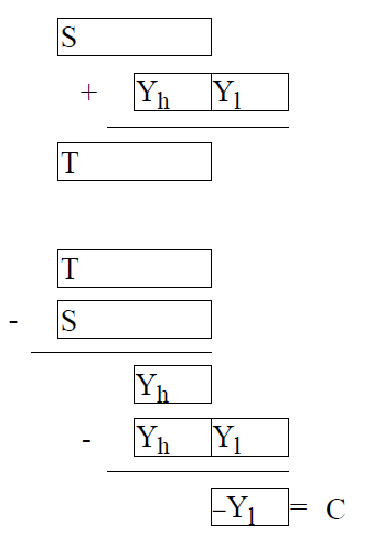
Each time a summand is added, there is a correction factor C which will be applied on the next loop. So first subtract the correction C computed in the previous loop from xjx_{j}xj, giving the corrected summand YYY. Then add this summand to the running sum SSS . The low order bits of Y (namely YlY_{l}Yl ) are lost in the sum. Next compute the high order bits of Y by computing T−ST-ST−S . When Y is subtracted from this, the low order bits of Y will be recovered. These are the bits that were lost in the first sum in the diagram. They become the correction factor for the next loop. A formal proof of Theorem 8, taken from Knuth 1981 page 572, appears in Section , "Theorem 14 and Theorem 8."
每次加入一个求和项时,会引入一个修正因子 CCC,并在下次循环中应用该因子:首先用当前求和项 xjx_jxj 减去上一次循环得到的修正因子 CCC,得到修正后的求和项 YYY;随后将 YYY 加入累加和 SSS,此过程中 YYY 的低阶位 YlY_lYl 会在求和中丢失;接着通过计算 T−ST-ST−S 得到 YYY 的高阶位 YhY_hYh,将 YYY 减去 YhY_hYh 即可恢复出求和中丢失的低阶位 YlY_lYl,该低阶位将作为下一次循环的修正因子。卡汉求和公式的形式化证明(引自克努斯 1981 年著作第 572 页)见本文 "定理 14 与定理 8" 小节。
Summary
总结
It is not uncommon for computer system designers to neglect the parts of a system related to floating-point. This is probably due to the fact that floating-point is given very little (if any) attention in the computer science curriculum. This in turn has caused the apparently widespread belief that floating-point is not a quantifiable subject, and so there is little point in fussing over the details of hardware and software that deal with it.
计算机系统设计者忽略系统中与浮点运算相关的部分,这一现象并不罕见。这可能是因为计算机科学的课程体系中,浮点运算的内容即便有涉及,也占比极低。这进而导致了一种普遍的错误认知:浮点运算并非一门可量化分析的学科,因此无需深究处理浮点运算的软硬件细节。
This paper has demonstrated that it is possible to reason rigorously about floating-point. For example, floating-point algorithms involving cancellation can be proven to have small relative errors if the underlying hardware has a guard digit, and there is an efficient algorithm for binary-decimal conversion that can be proven to be invertible, provided that extended precision is supported. The task of constructing reliable floating-point software is made much easier when the underlying computer system is supportive of floating-point. In addition to the two examples just mentioned (guard digits and extended precision), Section , "Systems Aspects," on page 211 of this paper has examples ranging from instruction set design to compiler optimization illustrating how to better support floating-point.
本文证明了对浮点运算进行严格的理论推导是可行的。例如:若硬件具备保护位,涉及相消误差的浮点算法可被证明具有较小的相对误差;若系统支持扩展精度,存在高效且可证明为可逆的二进制 - 十进制转换算法。当计算机系统对浮点运算提供良好支持时,开发高可靠性的浮点运算软件的难度会大幅降低。除了本文提到的保护位和扩展精度这两个例子, "系统层面" 小节中还给出了从指令集设计到编译器优化的多个实例,阐述了如何更好地为浮点运算提供系统支持。
The increasing acceptance of the IEEE floating-point standard means that codes that utilize features of the standard are becoming ever more portable. Section , "The IEEE Standard," on page 189, gave numerous examples illustrating how the features of the IEEE standard can be used in writing practical floating-point codes.
IEEE 浮点标准的认可度不断提高,这意味着利用该标准特性编写的代码具有更强的可移植性。本文 "IEEE 标准" 小节中,给出了大量实例,阐述了如何利用 IEEE 浮点标准的特性编写实用的浮点运算代码。
Acknowledgments
致谢
This article was inspired by a course given by W. Kahan at Sun Microsystems from May through July of 1988, which was very ably organized by David Hough of Sun. My hope is to enable others to learn about the interaction of floating-point and computer systems without having to get up in time to attend 8:00 a.m. lectures. Thanks are due to Kahan and many of my colleagues at Xerox PARC (especially John Gilbert) for reading drafts of this paper and providing many useful comments. Reviews from Paul Hilfinger and an anonymous referee also helped improve the presentation.
本文的创作灵感源于 W. 卡汉 1988 年 5 月至 7 月在太阳微系统公司开设的一门课程,该课程由太阳微系统公司的大卫・霍夫出色地组织策划。笔者希望能让更多人无需早起参加早 8 点的课程,也能学习到浮点运算与计算机系统的交互知识。感谢卡汉以及施乐帕洛阿尔托研究中心的多位同事(尤其是约翰・吉伯特),他们审阅了本文的草稿并提出了诸多宝贵意见;保罗・希尔芬格和一位匿名审稿人的评审建议,也对本文的表述优化起到了重要作用。
References
参考文献
Aho, Alfred V., Sethi, R., and Ullman J. D. 1986. Compilers: Principles, Techniques and Tools, Addison-Wesley, Reading, MA.
阿霍,阿尔弗雷德・V.、塞蒂,R.、厄尔曼,J.D.,1986,《编译原理:原理、技术与工具》,艾迪生 - 韦斯利出版社,美国马萨诸塞州雷丁市。
ANSI 1978. American National Standard Programming Language FORTRAN, ANSI Standard X3.9-1978, American National Standards Institute, New York, NY.
美国国家标准学会,1978,《美国国家标准程序设计语言 FORTRAN》,ANSI 标准 X3.9-1978,美国国家标准学会,美国纽约州纽约市。
Barnett, David 1987. A Portable Floating-Point Environment, unpublished manuscript.
巴内特,大卫,1987,《可移植的浮点运算环境》,未发表手稿。
CC
Brown, W. S. 1981. A Simple but Realistic Model of Floating-Point Computation, ACM Trans. on Math. Software 7 (4), pp. 445-480.
布朗,W.S.,1981,《一种简洁且贴合实际的浮点运算模型》,《美国计算机协会数学软件汇刊》,7 (4),445-480 页。
Cody, W. J et. al. 1984. A Proposed Radix- and Word-length-independent Standard for Floating-point Arithmetic, IEEE Micro 4 (4), pp. 86-100.
科迪,W.J. 等,1984,《一种独立于基数和字长的浮点运算标准提案》,《IEEE 微处理机》,4 (4),86-100 页。
Cody, W. J. 1988. Floating-Point Standards - Theory and Practice, in "Reliability in Computing: the role of interval methods in scientific computing", ed. by Ramon E. Moore, pp. 99-107, Academic Press, Boston, MA.
科迪,W.J.,1988,《浮点运算标准 ------ 理论与实践》,收录于《计算的可靠性:区间方法在科学计算中的作用》,雷蒙・E. 穆尔 主编,99-107 页,学术出版社,美国马萨诸塞州波士顿市。
Coonen, Jerome 1984. Contributions to a Proposed Standard for Binary FloatingPoint Arithmetic, PhD Thesis, Univ. of California, Berkeley.
库南,杰罗姆,1984,《对二进制浮点运算标准提案的研究贡献》,博士学位论文,美国加州大学伯克利分校。
Dekker, T. J. 1971. A Floating-Point Technique for Extending the Available Precision, Numer. Math. 18 (3), pp. 224-242.
德克尔,T.J.,1971,《一种提升可用精度的浮点运算技术》,《数值数学》,18 (3),224-242 页。
Demmel, James 1984. Underflow and the Reliability of Numerical Software, SIAM J. Sci. Stat. Comput. 5 (4), pp. 887-919.
德梅尔,詹姆斯,1984,《下溢与数值软件的可靠性》,《美国工业与应用数学学会科学与统计计算期刊》,5 (4),887-919 页。
Farnum, Charles 1988. Compiler Support for Floating-point Computation, Software-Practice and Experience, 18 (7), pp. 701-709.
法纳姆,查尔斯,1988,《编译器对浮点运算的支持》,《软件实践与经验》,18 (7),701-709 页。
Forsythe, G. E. and Moler, C. B. 1967. Computer Solution of Linear Algebraic Systems, Prentice-Hall, Englewood Cliffs, NJ.
福赛思,G.E.、莫勒,C.B.,1967,《线性代数系统的计算机求解方法》,普伦蒂斯 - 霍尔出版社,美国新泽西州恩格尔伍德克利夫斯市。
Goldberg, I. Bennett 1967. 27 Bits Are Not Enough for 8-Digit Accuracy, Comm. of the ACM. 10 (2), pp 105-106.
戈德堡,I. 贝内特,1967,《27 位二进制数无法满足 8 位十进制数的精度要求》,《美国计算机协会通讯》,10 (2),105-106 页。
Goldberg, David 1990. Computer Arithmetic, in "Computer Architecture: A Quantitative Approach", by David Patterson and John L. Hennessy, Appendix A, Morgan Kaufmann, Los Altos, CA.
戈德堡,大卫,1990,《计算机运算》,收录于《计算机体系结构:量化研究方法》,大卫・帕特森、约翰・L. 亨尼西 著,附录 A,摩根・考夫曼出版社,美国加利福尼亚州洛斯阿尔托斯市。
Golub, Gene H. and Van Loan, Charles F. 1989. Matrix Computations, 2nd edition,The Johns Hopkins University Press, Baltimore Maryland.
戈卢布,吉恩・H.、范洛恩,查尔斯・F.,1989,《矩阵计算》(第二版),约翰斯・霍普金斯大学出版社,美国马里兰州巴尔的摩市。
Graham, Ronald L. , Knuth, Donald E. and Patashnik, Oren. 1989. Concrete Mathematics, Addison-Wesley, Reading, MA, p.162.
格雷厄姆,罗纳德・L.、克努斯,唐纳德・E.、帕塔希尼克,奥伦,1989,《具体数学》,艾迪生 - 韦斯利出版社,美国马萨诸塞州雷丁市,162 页。
Hewlett Packard 1982. HP-15C Advanced Functions Handbook.
惠普公司,1982,《HP-15C 计算器高级功能手册》。
IEEE 1987. IEEE Standard 754-1985 for Binary Floating-point Arithmetic, IEEE, (1985). Reprinted in SIGPLAN 22 (2) pp. 9-25.
电气和电子工程师协会,1987,《IEEE 754-1985 二进制浮点运算标准》(1985 年发布),重印于《SIGPLAN 通讯》,22 (2),9-25 页。
Kahan, W. 1972. A Survey Of Error Analysis, in Information Processing 71, Vol 2, pp. 1214 - 1239 (Ljubljana, Yugoslavia), North Holland, Amsterdam.
卡汉,W.,1972,《误差分析综述》,收录于《1971 年信息处理大会论文集》,第二卷,1214-1239 页(南斯拉夫卢布尔雅那),北荷兰出版社,荷兰阿姆斯特丹市。
Kahan, W. 1986. Calculating Area and Angle of a Needle-like Triangle, unpublished manuscript.
卡汉,W.,1986,《针状三角形的面积与角度计算》,未发表手稿。
Kahan, W. 1987. Branch Cuts for Complex Elementary Functions, in "The State of the Art in Numerical Analysis", ed. by M.J.D. Powell and A. Iserles (Univ of Birmingham, England), Chapter 7, Oxford University Press, New York.
卡汉,W.,1987,《复初等函数的分支切割》,收录于《数值分析的发展现状》,M.J.D. 鲍威尔、A. 伊斯莱斯 主编(英国伯明翰大学),第七章,牛津大学出版社,美国纽约市。
Kahan, W. 1988. Unpublished lectures given at Sun Microsystems, Mountain View, CA.
卡汉,W.,1988,《在太阳微系统公司的未发表讲义》,美国加利福尼亚州山景城。
Kahan, W. and Coonen, Jerome T. 1982. The Near Orthogonality of Syntax, Semantics, and Diagnostics in Numerical Programming Environments, in "The Relationship Between Numerical Computation And Programming Languages", ed. by J. K. Reid, pp. 103-115, North-Holland, Amsterdam.
卡汉,W.、库南,杰罗姆・T.,1982,《数值编程环境中语法、语义与诊断的近似正交性》,收录于《数值计算与程序设计语言的关系》,J.K. 里德 主编,103-115 页,北荷兰出版社,荷兰阿姆斯特丹市。
Kahan, W. and LeBlanc, E. 1985. Anomalies in the IBM Acrith Package, Proc. 7th IEEE Symposium on Computer Arithmetic (Urbana, Illinois), pp. 322-331.
卡汉,W.、勒布朗,E.,1985,《IBM Acrith 数值库中的异常现象》,《第七届 IEEE 计算机算术研讨会论文集》(美国伊利诺伊州厄巴纳),322-331 页。
Kernighan, Brian W. and Ritchie, Dennis M. 1978. The C Programming Language, Prentice-Hall, Englewood Cliffs, NJ.
克尼汉,布赖恩・W.、里奇,丹尼斯・M.,1978,《C 程序设计语言》,普伦蒂斯 - 霍尔出版社,美国新泽西州恩格尔伍德克利夫斯市。
Kirchner, R. and Kulisch, U. 1987. Arithmetic for Vector Processors, Proc. 8th IEEE Symposium on Computer Arithmetic (Como, Italy), pp. 256-269.
基希纳,R.、库利施,U.,1987,《向量处理器的运算体系》,《第八届 IEEE 计算机算术研讨会论文集》(意大利科莫),256-269 页。
Knuth, Donald E., 1981. The Art of Computer Programming, Volume II, Second Edition, Addison-Wesley, Reading, MA.
克努斯,唐纳德・E.,1981,《计算机程序设计艺术》(第二卷,第二版),艾迪生 - 韦斯利出版社,美国马萨诸塞州雷丁市。
Kulisch, U. W., and Miranker, W. L. 1986. The Arithmetic of the Digital Computer: A New Approach, SIAM Review 28 (1), pp 1-36.
库利施,U.W.、米兰克,W.L.,1986,《数字计算机的运算体系:一种新方法》,《美国工业与应用数学学会述评》,28 (1),1-36 页。
Matula, D. W. and Kornerup, P. 1985. Finite Precision Rational Arithmetic: Slash Number Systems, IEEE Trans. on Comput. C-34 (1), pp 3-18.
马图拉,D.W.、科尔内鲁普,P.,1985,《有限精度有理数运算:斜杠数系》,《IEEE 计算机汇刊》,C-34 (1),3-18 页。
Nelson, G. 1991. Systems Programming With Modula-3, Prentice-Hall, Englewood Cliffs, NJ.
尼尔森,G.,1991,《使用 Modula-3 进行系统编程》,普伦蒂斯 - 霍尔出版社,美国新泽西州恩格尔伍德克利夫斯市。
Reiser, John F. and Knuth, Donald E. 1975. Evading the Drift in Floating-point Addition, Information Processing Letters 3 (3), pp 84-87.
赖泽,约翰・F.、克努斯,唐纳德・E.,1975,《规避浮点加法中的误差漂移》,《信息处理快报》,3 (3),84-87 页。
Sterbenz, Pat H. 1974. Floating-Point Computation, Prentice-Hall, Englewood Cliffs, NJ.
斯特本茨,帕特・H.,1974,《浮点运算》,普伦蒂斯 - 霍尔出版社,美国新泽西州恩格尔伍德克利夫斯市。
Swartzlander, Earl E. and Alexopoulos, Aristides G. 1975. The Sign/Logarithm Number System, IEEE Trans. Comput. C-24 (12), pp. 1238-1242.
斯沃茨兰德,厄尔・E.、亚历山普洛斯,阿里斯泰德斯・G.,1975,《符号 / 对数数系》,《IEEE 计算机汇刊》,C-24 (12),1238-1242 页。
Walther, J. S., 1971. A unified algorithm for elementary functions, Proceedings of the AFIP Spring Joint Computer Conf. 38, pp. 379-385.
沃尔瑟,J.S.,1971,《初等函数的统一算法》,《美国联邦信息处理学会春季联合计算机大会论文集》,38 卷,379-385 页。
未完,待校,待续......