LLAMA
- [1. Pre-RMSNorm替代Post-LayerNorm](#1. Pre-RMSNorm替代Post-LayerNorm)
- [2. GQA替代MHA,减少 KV 缓存。](#2. GQA替代MHA,减少 KV 缓存。)
- [3. 激活函数SwiGLU替代GeLU,提升前馈层表达力。](#3. 激活函数SwiGLU替代GeLU,提升前馈层表达力。)
- [4. RoPE 位置编码替换绝对位置编码,上下文窗口更长(4096 → 更大)。](#4. RoPE 位置编码替换绝对位置编码,上下文窗口更长(4096 → 更大)。)
基于Transformer的改动点:
1. Pre-RMSNorm替代Post-LayerNorm
RMSNorm
- 核心思想是仅对输入向量的均方根(RMS)进行归一化,不涉及均值中心化。
- 公式:
RMSNorm ( x ) = x 1 n ∑ i = 1 n x i 2 + ϵ ⊙ γ \text{RMSNorm}(\mathbf{x}) = \frac{\mathbf{x}}{\sqrt{\frac{1}{n}\sum_{i=1}^{n}x_i^2 + \epsilon}} \odot \mathbf{\gamma} RMSNorm(x)=n1∑i=1nxi2+ϵ x⊙γ
其中, x \mathbf{x} x 是输入向量。 n n n 是向量的维度。 ϵ \epsilon ϵ是极小值(如 10 − 6 10^{-6} 10−6),用于数值稳定性。 - 优点:
- 计算量小,不需要计算均值和标准差,显存/算力节约约 5%。
- 在大模型训练中更稳定,尤其在混合精度(FP16/BF16)下。
- 实现要点:在每个 Transformer 子层的 输入 前使用 RMSNorm,随后接 SwiGLU 与 注意力。
代码
python3
class LlamaRMSNorm(nn.Module):
    def __init__(self, hidden_size, eps=1e-6):
        super().__init__()
        self.weight = nn.Parameter(torch.ones(hidden_size))
        self.eps = eps

    def forward(self,hidden_states):
        rms = torch.sqrt(hidden_states.to(torch.float32).pow(2).mean(dim=-1,keepdim = True))
        return self.weight * (hidden_states/rms)
归一化在pre和post的区别
Post-LayerNorm:在每个子层(自注意力、前馈网络)输出之后进行归一化。
- 优势:
- 表达能力更强:子层的原始输出(未归一化)包含更丰富的数值分布,可能学习更复杂的模式。
- 适合浅层网络:在层数较少时(如原始Transformer的6层),梯度传播相对稳定。
- 劣势:
- 训练不稳定:深层网络中,残差连接后的输出可能因数值范围波动大,导致梯度爆炸/消失。
- 依赖精细调参:需配合学习率预热(Warmup)等技巧。
Pre-LayerNorm:在每个子层输入之前进行归一化。
- 优势:
- 训练更稳定:输入归一化后,子层计算的数值范围受控,梯度传播更平滑(传播路径更短)。
- 适合深层网络:减少梯度消失问题,支持训练百层以上的模型。
- 劣势:
- 表达能力受限:输入被强制归一化,可能损失部分信息多样性,需通过增加层数补偿。
2. GQA替代MHA,减少 KV 缓存。
- 动机:标准多头注意力的 Q、K、V 均为 head_num,导致 KV 缓存大小随 head_num 线性增长。
- 设计:
- 将 查询(Q) 分成 G 组,每组对应 head_num / G 个查询向量。
- 键/值(K/V) 仍保持完整的 head_num,但每组查询只与对应子集的 KV 交互。
- 实现细节:在 attention.py 中将 Q 维度 reshape 为 (batch, seq, G, head_per_group, d_head),随后按组进行点积。
代码
python3
class GroupedQueryAttention(nn.Module):
    def __init__(self, dim, num_heads, num_kv_heads = None, head_dim = None):
        """
        初始化分组查询注意力层

        参数:
            dim: 模型维度
            num_heads: 查询头数量
            num_kv_heads: 键值头数量(默认为 num_heads,即 MHA)
            head_dim: 每个头的维度(默认为 dim // num_heads)
        """
        super().__init__()
        self.num_heads = num_heads
        self.num_kv_heads = num_kv_heads if num_kv_heads else num_heads
        self.head_dim = head_dim if head_dim else dim//num_heads
        ## 重复因子
        self.n_rep = self.num_heads // self.num_kv_heads

        # 初始化权重矩阵
        self.wq = nn.Linear(dim, dim)  # 查询投影
        self.wk = nn.Linear(dim, self.num_kv_heads * self.head_dim)  # 键投影
        self.wv = nn.Linear(dim, self.num_kv_heads * self.head_dim)  # 值投影
        self.wo = nn.Linear(self.num_heads * self.head_dim, dim)  # 输出投影

    def _repeat_kv(self, x, n_rep):
        """重复KV头"""
        batch_size, seq_len, num_heads, head_dim = x.shape

        if n_rep == 1:
            return x

        # 扩展并重复
        x = x[:, :, :, None, :]  # [b, s, kv_h, 1, d]
        x = x.repeat(1, 1, 1 ,n_rep , 1)  # [b, s, kv_h, n_rep, d]
        x = x.reshape(batch_size, seq_len, num_heads * n_rep, head_dim)  # [b, s, h, d]
        return x

    def forward(self, x, mask=None):
        """
        前向传播

        参数:
            x: 输入张量 [batch_size, seq_len, dim]
            mask: 注意力掩码

        返回:
            输出张量 [batch_size, seq_len, dim]
        """
        batch_size, seq_len = x.shape[0], x.shape[1]
        # 1. 线性
        q, k, v = self.wq(x), self.wk(x), self.wv(x)

        # 2. 重塑为多头格式
        # q:[b,s,h,d], k:[b,s,kv_h,d], v:[b,s,kv_h,d]
        q = q.view(batch_size, seq_len, self.num_heads, -1)
        k = k.view(batch_size, seq_len, self.num_kv_heads, -1)
        v = v.view(batch_size, seq_len, self.num_kv_heads, -1)

        # 3. 重复KV头
        k = self._repeat_kv(k, self.n_rep)
        v = self._repeat_kv(v, self.n_rep) # [b,s,h,d]
        # 转换为 [b, h, s, d] 格式
        q, k, v = q.transpose(1,2), k.transpose(1,2), v.transpose(1,2)

        # 4. 计算注意力
        scores = torch.matmul(q, k.transpose(-2,-1))/(self.head_dim**0.5) # [b, h, s ,s]

        if mask is not None:
            scores = scores.masked_fill(mask == 0, -1e9)
        attn_weights = torch.softmax(scores, dim = -1)
        attn_output = torch.matmul(attn_weights, v)

        # 5. 合并多头并输出
        attn_output = attn_output.transpose(1,2).contiguous()
        attn_output = attn_output.view(batch_size, seq_len, - 1)
        output = self.wo(attn_output)
        return output

# 测试代码
def test_attention_modes():
    batch_size, seq_len, dim = 2, 10, 128
    x = torch.randn((batch_size, seq_len, dim))
    # 测试MHA模式
    mha = GroupedQueryAttention(dim, num_heads=8, num_kv_heads=8)
    print(f"MHA模式: num_heads={mha.num_heads}, num_kv_heads={mha.num_kv_heads}")
    y1 = mha(x)
    print(f'MHA模式:输入: {x.shape},输出:{y1.shape}')
    # 测试MQA模式
    mqa = GroupedQueryAttention(dim, num_heads=8, num_kv_heads=1)
    print(f"MQA模式: num_heads={mqa.num_heads}, num_kv_heads={mqa.num_kv_heads}")
    y2 = mqa(x)
    print(f'MHA模式:输入: {x.shape},输出:{y2.shape}')
    # 测试GQA模式
    gqa = GroupedQueryAttention(dim, num_heads=8, num_kv_heads=4)
    print(f"GQA模式: num_heads={gqa.num_heads}, num_kv_heads={gqa.num_kv_heads}, n_rep={gqa.n_rep}")
    y3 = gqa(x)
    print(f'MHA模式:输入: {x.shape},输出:{y3.shape}')
test_attention_modes()
3. 激活函数SwiGLU替代GeLU,提升前馈层表达力。
相比传统 GeLU,SwiGLU 在前馈网络中加入门控机制,提高表达能力并略微降低计算成本:
G e L U = x ϕ ( x ) ; S w i G L U = x ⋅ s w i s h ( x ) GeLU=x\phi(x);\quad SwiGLU= x \cdot swish(x) GeLU=xϕ(x);SwiGLU=x⋅swish(x)
- 为什么比 GELU 更好:
- 通过门控机制让网络自行决定信息流通路径,提升表达能力。
- 实验显示在相同计算量下,SwiGLU 可提升约 1‑2% 的 perplexity(困惑度)。
- 实现细节:在前馈网络的两层线性层之间插入 SwiGLU,保持隐藏维度不变。
代码
python3
# swish(xW+b)\ (xV+b)
class LlamaMLP(nn.Module):
    def __init__(self, hidden_size, middle_size):
        super().__init__()
        self.gate_proj = nn.Linear(hidden_size, middle_size, bias=False)
        self.up_proj = nn.Linear(hidden_size,middle_size,bias=False)
        self.down_proj = nn.Linear(middle_size, hidden_size, bias=False)
        self.activation = nn.SiLU()

    def forward(self, hidden_state):
        return self.down_proj(self.up_proj(hidden_state) * self.activation(self.gate_proj(hidden_state)))

middle_size = 256
MLP = LlamaMLP(hidden_size, middle_size)
output_x = MLP(input_x)
print('输入维度=',input_x.shape,'\t输出维度=', output_x.shape)
4. RoPE 位置编码替换绝对位置编码,上下文窗口更长(4096 → 更大)。
-
核心思想:将位置编码视为 二维旋转 操作,直接作用于查询/键的向量空间。
-
公式(2维简化):
x m = R m x , 其中 R m = ( cos m θ − sin m θ sin m θ cos m θ ) , θ p o s = p o s × 1 10000 − 2 i / d \mathbf{x}_m = \mathbf{R}_m \mathbf{x}, \quad \text{其中} \quad \mathbf{R}m = \begin{pmatrix} \cos m\theta & -\sin m\theta \\ \sin m\theta & \cos m\theta \end{pmatrix},\ \theta{pos}=pos \times \frac{1}{10000^{-2i/d}} xm=Rmx,其中Rm=(cosmθsinmθ−sinmθcosmθ), θpos=pos×10000−2i/d1 -
优势:
- 更好的外推性(长序列泛化)
- 原因:旋转矩阵的线性性质( R a R b = R a + b R_{a}R_{b}=R_{a+b} RaRb=Ra+b)使模型能处理远超训练时最大长度的序列。
- 对比:sin/cos编码在超长序列时需扩展位置索引,可能破坏位置间的关系。
sin/cos编码在超长序列中失效的本质原因是:
- 高频分量无法区分相邻位置;(波长: T = 2 π ∗ 10000 2 i / d , i T=2\pi*10000^{2i/d},i T=2π∗100002i/d,i为第i维特征,当 d d d较大时T较小,则相邻位置编码差异过小)
- 相对位置关系的外推超出训练范围;(位置内积: s i n ( m θ ) s i n ( n θ ) + c o s ( m θ ) c o s ( n θ ) = c o s ( ( m − n ) θ ) sin(mθ)sin(nθ)+cos(mθ)cos(nθ)=cos((m−n)θ) sin(mθ)sin(nθ)+cos(mθ)cos(nθ)=cos((m−n)θ), ( m − n ) θ (m-n)\theta (m−n)θ可能超出模型训练时见过的范围)
- 数值分布偏移破坏模型对位置的敏感性;(位置索引的增大导致编码值的数值分布偏离训练时的范围)
- 显式相对位置建模,适配长上下文
- 效果:直接通过旋转矩阵差计算相对位置,无需模型隐式学习,提升对位置敏感任务(如语言建模、机器翻译)的性能。
保持向量空间性质 - 特性:旋转不改变向量模长,仅调整方向,避免因位置编码叠加导致的数值尺度变化,提升训练稳定性。
- 效果:直接通过旋转矩阵差计算相对位置,无需模型隐式学习,提升对位置敏感任务(如语言建模、机器翻译)的性能。
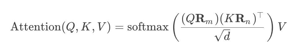
- 计算效率
实现:RoPE可融入注意力计算,无需额外存储位置编码矩阵,节省显存。例如,在计算 Q K T QK^{T} QKT 时直接应用旋转:
- 更好的外推性(长序列泛化)
代码
python3
######## 拆解版本
def compute_inv_freq(dim, base=10000):
    """ 计算逆频率向量 """
    indices = torch.arange(0,dim,2,dtype = torch.float)
    inv_freq = 1/(base **(indices/dim)) # 1/10000^{2j/d}, j = 0,1,...,d//2-1
    return inv_freq # [d//2,]

def compute_freqs(seq_len, inv_freq):
    """ 计算每个位置的角度矩阵 """
    positions = torch.arange(seq_len, dtype = torch.float).unsqueeze(1) # [seq_len, 1]
    freqs = torch.matmul(positions , inv_freq.unsqueeze(0))
    return freqs #[seq_len, d//2]

def compute_sin_cos(freqs):
    """ 计算余弦和正弦值 """ # e_{ix} = cosx + i sinx
    cos, sin = torch.cos(freqs), torch.sin(freqs)
    return cos, sin

def rotate_half(x):
    """ 将张量分成两半并旋转 ;参数:x: 输入张量,最后维度为 dim ;返回:旋转后的张量 """
    x1 = x[..., :x.shape[-1]//2]
    x2 = x[..., x.shape[-1]//2:]
    return torch.cat((-x2, x1), dim = -1)

def apply_rotary_emb(x, cos, sin):
    """
    应用旋转位置编码

    参数:
        x: 输入张量 [batch_size, seq_len, dim]
        cos: 余弦值 [seq_len, dim//2]
        sin: 正弦值 [seq_len, dim//2]

    返回:
        旋转后的张量
    """
    # 扩展 cos 和 sin 到与 x 相同的维度, 即 dim//2 扩展到 dim
    cos = cos.repeat_interleave(2, dim = -1) # 最后一个维度数据重复2次,[seq_len, d]
    sin = sin.repeat_interleave(2, dim = -1)
    # 应用旋转公式: x_rot = x * cos + rotate_half(x) * sin
    x_rot = x * cos + rotate_half(x) * sin ## 表示应用旋转后的attention输入向量,[x1',x2']=[x1 cos - x2sin, x2 cos + x1sin]
    return x_rot

dim = 64
seq_len = 20
batch_size = 4
inv_freq = compute_inv_freq(dim)
freqs = compute_freqs(seq_len,inv_freq)
cos, sin = compute_sin_cos(freqs)
q, k = torch.randn((batch_size, seq_len, dim)), torch.randn((batch_size, seq_len, dim))
q_rot, k_rot = apply_rotary_emb(q, cos, sin), apply_rotary_emb(k, cos, sin)
print(f'原始维度: {q.shape},{k.shape},\n旋转后维度:{q_rot.shape},{k_rot.shape}')

########### 融合版本
class Rope(nn.Module):
    def __init__(self, dim, seq_len, theta = 10000):
        super().__init__()
        self.dim = dim
        self.seq_len = seq_len
        self.theta = theta

    def permute_rote_matrix(self,dim, seq_len,theta):
        freqs = 1/(theta**(torch.arange(0, dim, 2)/dim))
        positions = torch.arange(seq_len, dtype = torch.float)
        freqs = torch.outer(positions, freqs) # [x,y]
        freq_cis = torch.polar(torch.ones_like(freqs), freqs) #[cosx + isinx, cosy + isiny]
        return freq_cis

    def apply_ratory_emb(self,x, freq_cis):
        """
        x:[batch_size, seq_len,dim]
        freq_cis:[seq_len, dim//2]
        """
        x_ = x.float().reshape(*x.shape[:-1], -1, 2)
        x_ = torch.view_as_complex(x_)  # 将最后两个维度变为实部、虚部
        x_out = torch.view_as_real(x_*freq_cis).flatten(2) # [batch_size, seq_len, dim],将dim = 2维度后进行flatten
        return x_out.type_as(x)

    def forward(self,x):
        freq_cis = self.permute_rote_matrix(self.dim, self.seq_len, self.theta)
        x_out = self.apply_ratory_emb(x, freq_cis)
        return x_out
dim = 64
seq_len = 20
batch_size = 4
Rope_emb = Rope(dim, seq_len)
q, k = torch.randn((batch_size, seq_len, dim)), torch.randn((batch_size, seq_len, dim))
q_rot, k_rot = Rope_emb(q), Rope_emb(k)
print(f'原始维度: {q.shape},{k.shape},\n旋转后维度:{q_rot.shape},{k_rot.shape}')