一致性哈希:不要相信教科书版本 如果你面试过分布式系统岗位,你一定画过那个经典的"哈希环"------一圈 232 的空间,节点散布其上,key 顺时针找到最近的节点。面试官满意地点头,你也觉得自己掌握了一致性哈希。
但我要告诉你:教科书版本的一致性哈希,在生产环境中几乎不可用。
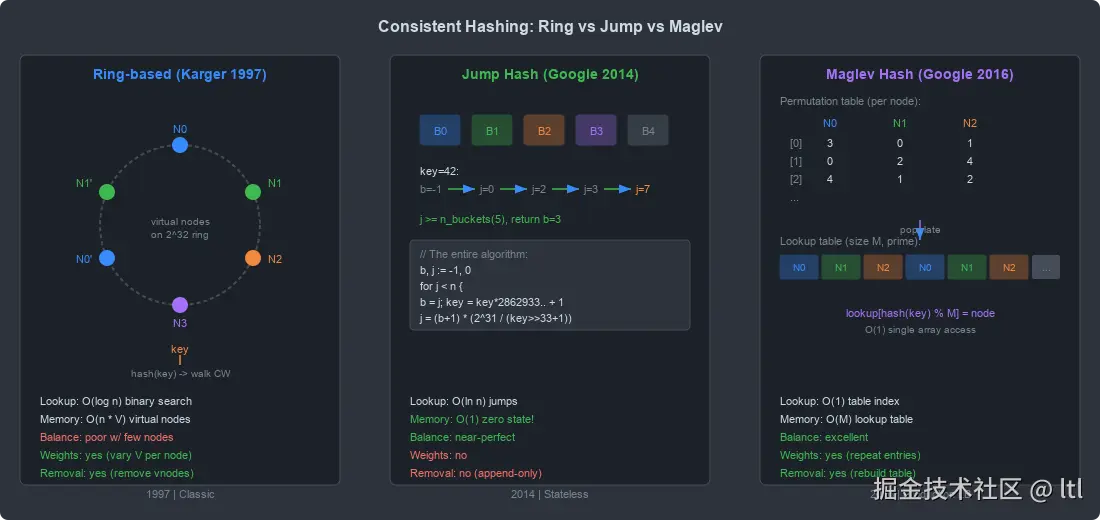
不是说它的思想有问题。Karger 等人 1997 年提出的一致性哈希,核心洞察是天才级的:通过把节点和 key 映射到同一个空间来最小化重映射。问题在于,教科书讲完哈希环和虚拟节点就停了,好像这就是终点。实际上这只是起点------一个有严重工程缺陷的起点。
虚拟节点的内存开销是 O(n⋅V),其中 V 通常需要 100-200 才能勉强保证均匀分布。1000 个节点就需要维护 10-20 万个虚拟节点的有序列表。查找需要二分搜索,每次 O(log(n⋅V))。节点变更时,所有副本都需要同步更新这个列表------在大规模集群中,这个元数据同步本身就是一个分布式一致性问题。
Google 显然很早就意识到了这些问题。2014 年,John Lamping 和 Eric Veach 发表了 Jump Consistent Hash:零内存开销、 O(lnn) 时间、近乎完美的均匀性,整个算法只有 5 行代码。2016 年,Google 又在 Maglev 论文中提出了一种基于置换表的哈希方案,专门为网络负载均衡设计: O(1) 查找、支持节点增删、负载均衡极其均匀。
本文不会只给你画一个哈希环然后收工。我会从经典方案的缺陷讲起,完整推导 Jump Hash 的数学原理,拆解 Maglev Hash 的置换表构造,给出 C 和 Go 的完整实现,最后用工程视角告诉你:在什么场景下,该用哪种一致性哈希。
一、问题定义:为什么需要一致性哈希
最朴素的方案及其灾难
假设你有 n 台缓存服务器,最简单的分片方式是:
ini
server = hash(key) % n这在 n 固定时工作得很好。但当你加一台服务器( n→n+1)或减一台服务器( n→n−1)时,几乎所有 key 的映射都会改变。具体来说, n/(n+1) 比例的 key 需要重新分配。对于 100 台服务器扩到 101 台,约 99% 的 key 需要迁移。
这在缓存场景下是灾难性的:所有缓存瞬间失效,后端数据库承受全量请求(cache stampede)。在存储场景下更糟------数据迁移的时间和带宽开销与集群规模成正比。
一致性哈希的核心目标
一致性哈希要解决的问题可以形式化为:
给定一个映射函数 f:K→N(从 key 空间到节点集合),当节点集合从 N 变为 N′ 时( ∣N△N′∣=1,即增加或删除一个节点),需要满足:
- 最小破坏性 (Minimal Disruption):只有 O(∣K∣/∣N∣) 个 key 需要重新映射
- 均衡性(Balance):每个节点分配到大致相等数量的 key
- 单调性(Monotonicity):当新节点加入时,key 只能从旧节点迁移到新节点,不能在旧节点之间迁移
这三个性质看起来直观,但同时满足它们并不容易。取模哈希满足第 2 条但完全违反第 1 条和第 3 条。
一个数学直觉
为什么取模哈希这么糟糕?因为 mod 运算对分母极其敏感。 hmod5 和 hmod6 的结果几乎没有关联。我们需要的是一种映射方式,使得分母的微小变化只影响一小部分输入的输出值。
一致性哈希的各种方案本质上都是在寻找这样一种"对分母变化鲁棒"的映射。它们的区别在于实现这种鲁棒性的具体机制,以及由此带来的不同 trade-off。
二、经典环形一致性哈希(Karger 1997)
哈希环的基本思想
1997 年,David Karger 等人在论文 Consistent Hashing and Random Trees 中提出了一致性哈希的经典方案。核心思想非常优雅:
- 将哈希空间视为一个环( [0,232) 首尾相连)
- 每个节点通过哈希映射到环上的一个点
- 每个 key 也通过哈希映射到环上的一个点
- key 沿顺时针方向找到的第一个节点,就是它的归属节点
c
#include <stdint.h>
#include <stdlib.h>
#include <string.h>

/* 简化的环形一致性哈希实现 */

typedef struct {
    uint32_t hash;
    int      node_id;
} vnode_t;

typedef struct {
    vnode_t *ring;
    int      ring_size;
    int      num_nodes;
    int      vnodes_per_node;
} ring_hash_t;

/* FNV-1a 哈希 */
static uint32_t fnv1a(const void *data, size_t len) {
    uint32_t h = 2166136261u;
    const uint8_t *p = (const uint8_t *)data;
    for (size_t i = 0; i < len; i++) {
        h ^= p[i];
        h *= 16777619u;
    }
    return h;
}

static int vnode_cmp(const void *a, const void *b) {
    uint32_t ha = ((const vnode_t *)a)->hash;
    uint32_t hb = ((const vnode_t *)b)->hash;
    if (ha < hb) return -1;
    if (ha > hb) return  1;
    return 0;
}

ring_hash_t *ring_create(int num_nodes, int vnodes_per_node) {
    ring_hash_t *rh = calloc(1, sizeof(*rh));
    rh->num_nodes = num_nodes;
    rh->vnodes_per_node = vnodes_per_node;
    rh->ring_size = num_nodes * vnodes_per_node;
    rh->ring = calloc(rh->ring_size, sizeof(vnode_t));

    int idx = 0;
    for (int n = 0; n < num_nodes; n++) {
        for (int v = 0; v < vnodes_per_node; v++) {
            /* 用 "node_id:vnode_index" 生成虚拟节点哈希 */
            char buf[64];
            int len = snprintf(buf, sizeof(buf), "%d:%d", n, v);
            rh->ring[idx].hash = fnv1a(buf, len);
            rh->ring[idx].node_id = n;
            idx++;
        }
    }

    /* 对环排序,以便二分查找 */
    qsort(rh->ring, rh->ring_size, sizeof(vnode_t), vnode_cmp);
    return rh;
}

int ring_lookup(ring_hash_t *rh, const void *key, size_t key_len) {
    uint32_t h = fnv1a(key, key_len);

    /* 二分查找:找到第一个 hash >= h 的虚拟节点 */
    int lo = 0, hi = rh->ring_size;
    while (lo < hi) {
        int mid = lo + (hi - lo) / 2;
        if (rh->ring[mid].hash < h)
            lo = mid + 1;
        else
            hi = mid;
    }

    /* 如果走到尾部,环绕到第一个节点 */
    if (lo == rh->ring_size)
        lo = 0;

    return rh->ring[lo].node_id;
}

void ring_destroy(ring_hash_t *rh) {
    free(rh->ring);
    free(rh);
}
虚拟节点的必要性
仅用物理节点映射到环上,分布极不均匀。设想 3 个节点分别映射到 0.1、 0.3、 0.35(归一化到 [0,1)),那么第一个节点负责 75% 的 key 空间( [0.35,0.1) 顺时针方向),而第三个节点只负责 5%。
虚拟节点(Virtual Nodes)是解决方案:每个物理节点在环上放置 V 个虚拟点。根据大数定律,当 V 足够大时,每个物理节点负责的 key 空间趋于均匀。
但"足够大"是多大?这正是问题所在。
均匀性的数学分析
假设 n 个节点各有 V 个虚拟节点,共 nV 个点均匀随机分布在环上。每个节点负责的期望 key 比例是 1/n,但方差是多少?
每个虚拟节点管辖的弧长服从参数为 nV 的指数分布的归一化版本。一个物理节点管辖的总弧长是其 V 个虚拟节点弧长之和。经过计算:
Var(1/nloadi)≈Vn
这意味着负载的标准差与 n/V 成正比。要让标准差低于期望负载的 ϵ 倍,需要:
V≥ϵ2n
对于 ϵ=0.05(5% 偏差),100 个节点需要 V=40000。这 400 万个虚拟节点的有序列表在内存中占据数十 MB,而且每次节点变更都要重新排序。
实际系统中通常取 V=100∼200 作为折中,接受约 10-15% 的负载不均。但这种"凑合用"的做法让人不太舒服。
三、教科书版本的工程缺陷
在生产环境中部署环形一致性哈希后,你会发现教科书没有提到的问题远不止负载不均。
缺陷一:内存开销
每个虚拟节点至少需要存储一个哈希值(4-8 字节)和一个节点标识。假设 1000 个物理节点、每个 150 个虚拟节点:
- 虚拟节点总数:150,000
- 每个条目:8 字节哈希 + 4 字节节点 ID = 12 字节
- 总内存:~1.8 MB(仅哈希环)
这看起来不多,但考虑到:
- 每个客户端都需要持有这份数据的完整副本
- 在微服务架构中,可能有数千个客户端实例
- 总内存消耗 = 1.8 MB * 客户端数量
缺陷二:元数据同步
当节点增删时,所有客户端都必须更新自己的哈希环副本。这引入了一个分布式一致性问题:在更新传播的过程中,不同客户端可能对同一个 key 路由到不同节点。
你需要一个额外的协调机制(通常是 ZooKeeper 或 etcd)来通知所有客户端。而且你还需要考虑更新的原子性------部分更新的哈希环可能导致负载剧烈不均。
缺陷三:热点放大
虚拟节点在环上的位置是伪随机的,不保证物理上的均匀间隔。在极端情况下,一个物理节点的多个虚拟节点可能"聚堆",导致该节点的负载远低于平均水平,而相邻节点被压垮。
更糟的是,当一个节点故障下线时,它的负载全部转移到环上的下一个节点------而不是均匀分散到所有存活节点。这意味着一次故障可能引发级联故障。
缺陷四:查找性能
二分查找的时间复杂度是 O(log(nV))。对于 150,000 个虚拟节点,约需 17 次比较。每次比较涉及一次内存访问,在 cache miss 的情况下(虚拟节点列表可能无法完全放入 L1/L2 缓存),单次查找可能需要 200-500 纳秒。
对于网络负载均衡器这种每秒需要处理数百万包的场景,这个延迟是不可接受的。
缺陷五:缺乏形式化保证
环形一致性哈希的均匀性依赖于哈希函数的随机性和虚拟节点的数量,缺乏严格的理论上界。你无法提前计算"给定 n 和 V,最大负载比率保证不超过 X"------只能通过经验和模拟来调参。
这在需要 SLA 保证的生产环境中是一个严重的缺陷。
四、Jump Consistent Hash:零内存的优雅算法
背景
2014 年,Google 的 John Lamping 和 Eric Veach 发表了论文 A Fast, Minimal Memory, Consistent Hash Algorithm。这篇论文提出的 Jump Consistent Hash 是我见过的最优雅的算法之一:
- 零状态:不需要任何数据结构
- O(lnn) 时间
- 近乎完美的均匀性
- 完整实现只有 7 行 C 代码
核心思想
Jump Hash 的思想极其巧妙。它不维护哈希环,而是直接通过一个确定性的"跳跃"过程,为每个 key 计算出它应该归属的桶编号。
设想桶数从 1 逐步增加到 n。当桶数从 b 增加到 b+1 时,每个 key 有 1/(b+1) 的概率被重新分配到新桶。Jump Hash 的巧妙之处在于:它不逐步模拟这个过程,而是计算"下一次跳跃会发生在哪里",直接跳过大量不需要重分配的步骤。
数学推导
让我们从头推导这个算法。
定义 : ch(k,n) 表示 key k 在 n 个桶中被分配到的桶编号。
性质 1 :当桶数从 n 增加到 n+1 时,每个 key 以概率 1/(n+1) 被重新分配到桶 n(新桶),以概率 n/(n+1) 保持原来的桶。
这保证了最小破坏性:从 n 到 n+1,只有约 1/(n+1) 的 key 发生迁移。
逐步构建:
假设我们从 1 个桶开始,逐步增加到 n 个桶。对于每个 key k,定义一个与 k 相关的伪随机序列 r1,r2,...,其中 rj∈[0,1)。当桶数从 j 增加到 j+1 时,key k 跳到新桶当且仅当 rj<1/(j+1)。
朴素实现需要遍历 j=1,2,...,n−1,这是 O(n) 的。
关键优化------跳跃:
如果 key 当前在桶 b,我们想知道:下一次它会跳到新桶是在桶数增加到几的时候?
设当前桶数为 j+1(key 在桶 b=j),下一次跳跃发生在桶数变为 j′ 时。在 j+1 到 j′−1 之间的每一步,key 都没有跳跃。不跳跃的概率是:
P(不跳)=j+2j+1⋅j+3j+2⋯j′j′−1=j′j+1
因此跳跃发生在 j′ 的概率是 j′j+1⋅j′+11,而 j′>j′′ 的累积概率是 j′′+1j+1。
我们可以用逆采样法:生成一个均匀随机数 r∈[0,1),令 j′j+1=r,解得:
j′=⌊(j+1)/r⌋
这就是"跳跃"的来源------我们不需要逐步检查每个桶数,而是一步跳到下一个会发生重分配的桶数。
时间复杂度分析:
每次跳跃后, j 至少增长到 (j+1)/r 的期望值。 E1/r=∫011/rdr 发散,但 E⌊(j+1)/r⌋ 的增长率意味着从 1 跳到 n 的期望步数是 O(lnn)。
直觉上,每步的期望增长因子约为 E⌊1/r⌋≈e(自然对数的底),所以步数约为 lnn。
完整实现
以下是论文中给出的 C 实现(加上我的注释):
c
#include <stdint.h>

/*
 * Jump Consistent Hash
 *
 * 输入:key   - 64 位哈希值
 *       num_buckets - 桶的数量(>= 1)
 * 输出:[0, num_buckets) 范围内的桶编号
 *
 * 性质:
 *   - 当 num_buckets 从 n 变为 n+1 时,约 1/(n+1) 的 key 改变映射
 *   - 完美均匀分布
 *   - O(ln(num_buckets)) 时间,O(1) 空间
 */
int32_t jump_consistent_hash(uint64_t key, int32_t num_buckets) {
    int64_t b = -1, j = 0;
    while (j < num_buckets) {
        b = j;
        key = key * 2862933555777941757ULL + 1;
        j = (int64_t)((b + 1) * ((double)(1LL << 31) /
            (double)((key >> 33) + 1)));
    }
    return (int32_t)b;
}
让我逐行解析:
b = -1, j = 0:b是上一次跳跃的目标桶,j是本次跳跃的候选目标while (j < num_buckets):当候选目标还在有效范围内b = j:记录有效的目标桶key = key * 2862933555777941757ULL + 1:线性同余生成器产生伪随机数(这个常数是精心选择的,具有良好的统计特性)j = (b + 1) * (2^31 / (key >> 33 + 1)):这就是 j′=⌊(b+1)/r⌋ 的实现,其中 r 来自伪随机数的高位
这个算法精妙到令人叹服:没有任何数据结构、没有排序、没有二分查找。完全是纯计算。
Go 实现
go
package jumphash

// JumpHash 实现 Jump Consistent Hash 算法。
// key 是 64 位哈希值,numBuckets 是桶数。
// 返回 [0, numBuckets) 范围内的桶编号。
func JumpHash(key uint64, numBuckets int32) int32 {
    var b, j int64
    b = -1
    j = 0
    for j < int64(numBuckets) {
        b = j
        key = key*2862933555777941757 + 1
        j = int64(float64(b+1) *
            (float64(int64(1)<<31) / float64((key>>33)+1)))
    }
    return int32(b)
}
Jump Hash 的局限
Jump Hash 近乎完美,但有一个致命限制:它只支持桶的追加和从尾部移除。你不能删除中间的一个桶。
具体来说,如果你有桶 {0,1,2,3,4},移除桶 2 后变成 {0,1,3,4}------但 Jump Hash 不支持这种操作。它只能从 5 个桶变成 4 个桶,相当于移除了桶 4。
这在实际中意味着:如果集群中一台服务器故障,你不能直接把它从桶列表中删除。你必须用一个映射层把"逻辑桶"映射到"物理服务器"------而这个映射层本身就需要分布式一致性。
所以 Jump Hash 最适合的场景是:节点数量单调递增或很少变化的情况,比如分布式存储的 shard 分配。
五、Multi-probe Consistent Hashing:用 CPU 换内存
设计思想
2015 年,Appleton 和 O'Reilly 提出了 Multi-probe Consistent Hashing。它的思想是:
- 每个节点只在环上放置一个点(不需要虚拟节点)
- 查找时,用 key 生成 k 个探测点(probe),选择距离最近节点最近的那个探测点对应的节点
这本质上是用查找时的 CPU 开销(多次哈希计算)来换取存储时的内存开销(不需要虚拟节点)。
算法
go
package multiprobe

import (
    "hash/crc64"
    "math"
    "encoding/binary"
)

type MultiProbeHash struct {
    nodes     []uint64  // 每个节点在环上的哈希值
    nodeIDs   []int     // 节点 ID
    numProbes int       // 探测次数
}

func New(nodeIDs []int, numProbes int) *MultiProbeHash {
    mph := &MultiProbeHash{
        nodes:     make([]uint64, len(nodeIDs)),
        nodeIDs:   make([]int, len(nodeIDs)),
        numProbes: numProbes,
    }
    tab := crc64.MakeTable(crc64.ECMA)
    for i, id := range nodeIDs {
        var buf [4]byte
        binary.LittleEndian.PutUint32(buf[:], uint32(id))
        mph.nodes[i] = crc64.Checksum(buf[:], tab)
        mph.nodeIDs[i] = id
    }
    return mph
}

func (mph *MultiProbeHash) Lookup(key []byte) int {
    tab := crc64.MakeTable(crc64.ECMA)
    bestDist := uint64(math.MaxUint64)
    bestNode := 0

    for p := 0; p < mph.numProbes; p++ {
        /* 为每次探测生成不同的哈希值 */
        var buf [len(key) + 4]byte
        copy(buf[:], key)
        binary.LittleEndian.PutUint32(buf[len(key):], uint32(p))
        probeHash := crc64.Checksum(buf[:len(key)+4], tab)

        /* 找到最近的节点 */
        for i, nodeHash := range mph.nodes {
            var dist uint64
            if probeHash >= nodeHash {
                dist = probeHash - nodeHash
            } else {
                dist = nodeHash - probeHash
            }
            /* 环形距离 */
            if dist > math.MaxUint64/2 {
                dist = math.MaxUint64 - dist + 1
            }
            if dist < bestDist {
                bestDist = dist
                bestNode = mph.nodeIDs[i]
            }
        }
    }
    return bestNode
}
均匀性分析
论文证明,使用 k 个探测点时,最大负载比率(最重节点负载 / 平均负载)的上界约为:
1+kϵ
其中 ϵ 是一个与节点数相关的常数。实践中, k=21 个探测点就能达到与 700 个虚拟节点相当的均匀性,但内存开销从 O(700n) 降到了 O(n)。
代价是每次查找需要计算 21 次哈希并遍历所有节点,时间复杂度 O(kn)。不过对于节点数较少(< 100)的场景,这完全可以接受。
六、Maglev Hashing:Google 的网络负载均衡之王
背景
2016 年,Google 发表了论文 Maglev: A Fast and Reliable Software Network Load Balancer。Maglev 是 Google 的软件网络负载均衡器,处理 Google 几乎所有面向用户的流量。
Maglev Hash 是论文中提出的一致性哈希方案,专门为网络负载均衡设计。它的核心特征:
- O(1) 查找(单次数组索引)
- 支持节点的动态增删
- 极其均匀的负载分布
- 构建查找表的时间是 O(M⋅logM)( M 是表大小)
算法原理
Maglev Hash 的核心是一个大小为 M 的查找表( M 必须是质数,通常取 65537 或更大的质数)。查找时,只需计算 lookup_table[hash(key) % M] 即可得到目标节点。
查找表的构建过程如下:
步骤 1:为每个节点生成一个置换序列。
每个节点 i 有两个哈希值:
- offseti=h1(namei)modM
- skipi=h2(namei)mod(M−1)+1
节点 i 的偏好列表(置换序列)为: permutationij=(offseti+j⋅skipi)modM
因为 M 是质数且 skipi∈1,M−1,所以这个序列恰好覆盖 [0,M) 的所有值(是 ZM 的一个完整遍历)。
步骤 2:轮流填充查找表。
节点按轮次(Round-Robin)依次尝试填充查找表的空位。每个节点按自己的偏好顺序选择位置。如果某个位置已被其他节点占据,就跳过,尝试下一个偏好位置。
这个过程保证了:
- 最终每个位置恰好被一个节点占据
- 每个节点占据约 M/n 个位置( n 是节点数)
- 当一个节点下线时,它的位置被其他节点"接管",影响范围最小化
C 实现
c
#include <stdint.h>
#include <stdlib.h>
#include <string.h>
#include <stdio.h>

#define MAGLEV_TABLE_SIZE 65537  /* 质数 */

typedef struct {
    int32_t  *lookup;            /* 查找表 */
    int32_t   table_size;        /* M(质数) */
    int32_t   num_nodes;
    uint32_t *offset;            /* 每个节点的 offset */
    uint32_t *skip;              /* 每个节点的 skip */
} maglev_t;

/* DJB2 哈希 */
static uint32_t djb2(const char *str, uint32_t seed) {
    uint32_t h = 5381 + seed;
    int c;
    while ((c = *str++))
        h = ((h << 5) + h) + c;
    return h;
}

maglev_t *maglev_create(const char **node_names, int num_nodes,
                         int table_size) {
    maglev_t *mg = calloc(1, sizeof(*mg));
    mg->table_size = table_size;
    mg->num_nodes  = num_nodes;
    mg->lookup     = malloc(sizeof(int32_t) * table_size);
    mg->offset     = malloc(sizeof(uint32_t) * num_nodes);
    mg->skip       = malloc(sizeof(uint32_t) * num_nodes);

    for (int i = 0; i < num_nodes; i++) {
        mg->offset[i] = djb2(node_names[i], 0) % table_size;
        mg->skip[i]   = djb2(node_names[i], 42) % (table_size - 1) + 1;
    }

    /* 填充查找表 */
    for (int i = 0; i < table_size; i++)
        mg->lookup[i] = -1;

    /* next[i] 记录节点 i 在偏好列表中的当前位置 */
    int *next = calloc(num_nodes, sizeof(int));
    int filled = 0;

    while (filled < table_size) {
        for (int i = 0; i < num_nodes && filled < table_size; i++) {
            /* 节点 i 按偏好顺序寻找空位 */
            uint32_t pos = (mg->offset[i] +
                           (uint64_t)next[i] * mg->skip[i]) % table_size;
            while (mg->lookup[pos] != -1) {
                next[i]++;
                pos = (mg->offset[i] +
                      (uint64_t)next[i] * mg->skip[i]) % table_size;
            }
            mg->lookup[pos] = i;
            next[i]++;
            filled++;
        }
    }

    free(next);
    return mg;
}

int32_t maglev_lookup(maglev_t *mg, const void *key, size_t key_len) {
    uint32_t h = 5381;
    const uint8_t *p = (const uint8_t *)key;
    for (size_t i = 0; i < key_len; i++)
        h = ((h << 5) + h) + p[i];
    return mg->lookup[h % mg->table_size];
}

void maglev_destroy(maglev_t *mg) {
    free(mg->lookup);
    free(mg->offset);
    free(mg->skip);
    free(mg);
}
Go 实现
go
package maglev

import (
    "hash/fnv"
)

const DefaultTableSize = 65537 // 质数

type Maglev struct {
    lookup    []int32
    tableSize int
    nodes     []string
    offset    []uint32
    skip      []uint32
}

func hashStr(s string, seed uint32) uint32 {
    h := fnv.New32a()
    b := [4]byte{byte(seed), byte(seed >> 8),
                  byte(seed >> 16), byte(seed >> 24)}
    h.Write(b[:])
    h.Write([]byte(s))
    return h.Sum32()
}

func New(nodes []string, tableSize int) *Maglev {
    m := &Maglev{
        lookup:    make([]int32, tableSize),
        tableSize: tableSize,
        nodes:     nodes,
        offset:    make([]uint32, len(nodes)),
        skip:      make([]uint32, len(nodes)),
    }

    for i, name := range nodes {
        m.offset[i] = hashStr(name, 0) % uint32(tableSize)
        m.skip[i] = hashStr(name, 42)%uint32(tableSize-1) + 1
    }

    m.populate()
    return m
}

func (m *Maglev) populate() {
    for i := range m.lookup {
        m.lookup[i] = -1
    }

    n := len(m.nodes)
    next := make([]int, n)
    filled := 0

    for filled < m.tableSize {
        for i := 0; i < n && filled < m.tableSize; i++ {
            pos := (uint64(m.offset[i]) +
                uint64(next[i])*uint64(m.skip[i])) % uint64(m.tableSize)
            for m.lookup[pos] != -1 {
                next[i]++
                pos = (uint64(m.offset[i]) +
                    uint64(next[i])*uint64(m.skip[i])) % uint64(m.tableSize)
            }
            m.lookup[pos] = int32(i)
            next[i]++
            filled++
        }
    }
}

func (m *Maglev) Lookup(key []byte) int {
    h := fnv.New32a()
    h.Write(key)
    idx := h.Sum32() % uint32(m.tableSize)
    return int(m.lookup[idx])
}

// RemoveNode 移除一个节点并重建查找表。
// 返回新的 Maglev 实例。
func RemoveNode(m *Maglev, nodeIdx int) *Maglev {
    newNodes := make([]string, 0, len(m.nodes)-1)
    for i, name := range m.nodes {
        if i != nodeIdx {
            newNodes = append(newNodes, name)
        }
    }
    return New(newNodes, m.tableSize)
}
Maglev Hash 的性质
最小破坏性 :当一个节点下线时,它在查找表中占据的约 M/n 个条目需要被重新分配。由于每个节点的偏好序列是独立生成的,这些空位会被其他节点"自然地"按偏好顺序接管。实验表明,实际重映射比例非常接近理论最优值 1/n。
均匀性 :因为查找表是通过轮次填充的,每个节点占据的条目数至多差 1( ⌊M/n⌋ 或 ⌈M/n⌉)。这比环形一致性哈希的统计近似要精确得多。
查找性能:单次哈希 + 单次数组访问。在现代 CPU 上,如果查找表能放入 L2/L3 缓存(65537 个 int32 = 256 KB),查找延迟约 10-30 纳秒。
七、Rendezvous Hashing:最高随机权重
HRW 的朴素优雅
Rendezvous Hashing(也叫 Highest Random Weight,HRW)由 Thaler 和 Ravishankar 在 1998 年提出。它可能是概念上最简单的一致性哈希:
对于每个 key,计算它与每个节点的"权重": wi=h(key,nodei),选择权重最高的节点。
c
#include <stdint.h>

/* 简化的 Rendezvous / HRW 哈希 */

static uint64_t hrw_hash(const void *key, size_t key_len,
                         uint32_t node_id) {
    /* 使用 key 和 node_id 共同作为输入 */
    uint64_t h = 14695981039346656037ULL;  /* FNV offset basis */
    const uint8_t *p = (const uint8_t *)key;
    for (size_t i = 0; i < key_len; i++) {
        h ^= p[i];
        h *= 1099511628211ULL;
    }
    /* 混入 node_id */
    h ^= node_id;
    h *= 1099511628211ULL;
    h ^= (node_id >> 8);
    h *= 1099511628211ULL;
    return h;
}

int rendezvous_lookup(const void *key, size_t key_len,
                      const uint32_t *node_ids, int num_nodes) {
    uint64_t max_weight = 0;
    int best = 0;
    for (int i = 0; i < num_nodes; i++) {
        uint64_t w = hrw_hash(key, key_len, node_ids[i]);
        if (w > max_weight) {
            max_weight = w;
            best = i;
        }
    }
    return best;
}
HRW 的性质
一致性:当移除一个节点时,只有之前分配给该节点的 key 会被重新分配------因为其他 key 的 "最高权重" 节点没有变。这是完美的最小破坏性。
均匀性:假设哈希函数足够随机,每个节点成为"最高权重"的概率相等,因此分布完美均匀。
致命缺陷------ O(n) 查找:每次查找需要遍历所有节点。当节点数很大时(比如上千个),这个开销不可接受。
不过对于节点数较少的场景(10-50 个),HRW 是一个极好的选择:实现简单、理论性质完美、支持任意增删。很多 CDN 系统内部使用 HRW 来做源站选择。
加权 Rendezvous
HRW 天然支持加权:将权重 wi 缩放为 wi1/weighti 即可。权重越大的节点,缩放后的值越可能是最大的。
go
package rendezvous

import (
    "hash/fnv"
    "math"
    "encoding/binary"
)

type WeightedNode struct {
    ID     string
    Weight float64
}

func WeightedLookup(key []byte, nodes []WeightedNode) int {
    best := -1
    bestScore := -math.MaxFloat64

    for i, node := range nodes {
        h := fnv.New64a()
        h.Write(key)
        h.Write([]byte(node.ID))
        hashVal := h.Sum64()

        /* 将哈希值归一化到 (0, 1),再取 weight 次幂的对数 */
        normalized := float64(hashVal) / float64(math.MaxUint64)
        if normalized == 0 {
            normalized = 1e-18
        }
        score := math.Log(normalized) / node.Weight

        if score > bestScore {
            bestScore = score
            best = i
        }
    }
    _ = binary.LittleEndian /* suppress unused import */
    return best
}
八、算法对比:一张表说清楚
以下是四种主流一致性哈希算法的全面对比:
| 维度 | Ring(Karger) | Jump Hash | Maglev Hash | Rendezvous(HRW) |
|---|---|---|---|---|
| 提出时间 | 1997 | 2014 | 2016 | 1998 |
| 查找时间 | O(log(nV)) | O(lnn) | O(1) | O(n) |
| 内存开销 | O(nV) | O(1) | O(M) | O(n) |
| 均匀性 | 依赖 V,一般 | 近乎完美 | 非常好( ±1 条目) | 完美 |
| 最小破坏性 | 约 1/n(理论) | 精确 1/n | 接近 1/n | 精确 1/n |
| 支持加权 | 是(调整 V) | 否 | 是(重复填充) | 是(缩放权重) |
| 支持任意删除 | 是 | 否(仅尾部) | 是(重建表) | 是 |
| 实现复杂度 | 中等 | 极低 | 中等 | 极低 |
| 适用节点规模 | 中等(100-1000) | 大(1-10000+) | 中等(10-1000) | 小(10-100) |
| 构建/重建代价 | O(nVlog(nV)) | 无 | O(M⋅n) | 无 |
选择指南
这张表的关键洞察是:没有银弹。每种算法在不同维度上做了不同的 trade-off。
- 如果你的节点只会增加不会减少(如分布式存储的 shard),Jump Hash 是最佳选择
- 如果你需要极低延迟的查找且节点会动态变化(如负载均衡),Maglev Hash 是首选
- 如果你的节点数很少且需要加权(如多数据中心的流量调度),Rendezvous 是最简洁的方案
- 如果你需要兼容现有生态(如 Memcached 客户端),环形一致性哈希可能是唯一选择
九、真实系统中的一致性哈希
Memcached:经典环形
Memcached 的客户端库(如 libmemcached、ketama)使用最经典的环形一致性哈希。Ketama 最初由 Last.fm 开发,使用 MD5 哈希,每个节点 100-200 个虚拟节点。
这是一个"够用就行"的典型案例。Memcached 的节点数通常不多(几十到一两百),客户端只需要在初始化时构建哈希环,查找性能不是瓶颈。
Cassandra:token ring
Cassandra 使用一种改进的环形分区方案。与经典一致性哈希不同,Cassandra 的 token ring 中每个节点负责一个明确的 token 范围,由 partitioner(如 Murmur3Partitioner)决定。
在 Cassandra 3.0 之前,添加新节点需要手动选择 token 来平衡负载。3.0 引入的 vnode 机制允许每个节点持有多个不连续的 token 范围,本质上就是虚拟节点------但由集群自动管理。
Nginx:加权一致性哈希
Nginx 的 upstream 模块支持 hash ... consistent 指令,使用 Ketama 风格的环形一致性哈希。它支持权重:权重为 w 的节点获得 160w 个虚拟节点。
nginx
upstream backend {
    hash $request_uri consistent;
    server 10.0.0.1:8080 weight=3;
    server 10.0.0.2:8080 weight=2;
    server 10.0.0.3:8080 weight=1;
}
Envoy:Ring Hash + Maglev 双支持
Envoy Proxy 同时支持环形一致性哈希和 Maglev Hash,用户可以通过配置选择。
对于环形哈希,Envoy 默认每个节点 1024 个虚拟节点(远高于 Ketama 的 100-200),代价是更多内存和更慢的构建速度。
对于 Maglev,Envoy 使用 65537 作为表大小。Envoy 的文档明确指出:Maglev 在稳定性(节点变更时的重映射比例)上不如环形哈希,但查找速度快得多,适合对延迟敏感的场景。
Google Maglev:生产级网络负载均衡
Google 的 Maglev 负载均衡器使用 Maglev Hash 将入站连接分配到后端服务器。Maglev 运行在 Google 数据中心的边缘,每台机器处理高达 10 Gbps 的流量。
Maglev Hash 的 O(1) 查找是关键:在网络负载均衡中,每个数据包都需要查找,而非每个连接。以 64 字节的最小包大小计算,10 Gbps 意味着每秒约 2000 万个包。即使 50 纳秒的查找延迟,在这个规模下也会消耗一个 CPU 核心的大部分时间。
DynamoDB 和 Amazon 的方案
Amazon 的 Dynamo 论文(2007)使用了改进的一致性哈希。与经典方案不同,Dynamo 给每个节点分配多个等大小的 token 范围(而非随机位置的虚拟节点),并通过一个 gossip 协议同步这些范围的分配。这种"策略三"方案解决了虚拟节点位置随机导致的不均匀问题。
十、工程踩坑表
在生产环境中实现一致性哈希,以下是我见过(和自己踩过)的常见陷阱:
| 序号 | 陷阱 | 后果 | 对策 |
|---|---|---|---|
| 1 | 哈希函数选择不当(如使用 CRC32 或 Java 的 hashCode) | 分布严重不均,某些节点负载是平均值的 3-5 倍 | 使用 xxHash、FNV-1a、Murmur3 等分布良好的哈希函数 |
| 2 | 虚拟节点数量不足(< 50) | 节点间负载差异 > 20% | 至少使用 100-200 个虚拟节点;或者换用 Jump/Maglev |
| 3 | 节点变更时未考虑连接排空(drain) | 正在处理的请求被中断,导致错误率飙升 | 变更前先标记节点为 draining,等待现有连接完成后再修改哈希环 |
| 4 | 哈希环在多个副本间不一致 | 同一个 key 在不同客户端被路由到不同节点,导致缓存命中率暴跌 | 使用版本号或 epoch 机制,确保所有客户端使用相同版本的哈希环 |
| 5 | Maglev 表大小选择非质数 | 置换序列无法覆盖所有位置,填充过程死循环 | 表大小必须是质数;推荐 65537( 216+1) |
| 6 | Jump Hash 用于需要节点删除的场景 | 无法正确处理中间节点故障,导致大量 key 重映射 | Jump Hash 仅适用于追加场景;需要删除时改用 Maglev 或 Ring |
| 7 | 未处理哈希碰撞(两个虚拟节点哈希值相同) | 一个虚拟节点"消失",其负载转移到相邻节点 | 使用 128 位哈希或在排序后检测碰撞;碰撞时用备用哈希 |
| 8 | 节点权重变更触发全量重建 | 在大集群中重建耗时数秒,期间查找可能不一致 | 支持增量更新;或使用 double-buffer 方案无缝切换 |
| 9 | 未考虑热点 key 的特殊处理 | 单个热点 key 压垮一个节点,一致性哈希无法解决 | 热点 key 需要在应用层做复制或分裂;一致性哈希不解决热点问题 |
| 10 | 跨数据中心部署时忽略了网络分区 | 分区期间不同数据中心的哈希环状态不同 | 每个数据中心独立的哈希环 + 跨中心的路由层 |
十一、性能基准
为了让对比更直观,以下是在同一台机器上(AMD Ryzen 9 7950X,DDR5-5600)测量的各算法性能数据。节点数 100,key 为随机 64 位整数。
ini
算法                   查找延迟(ns)    内存(KB)    构建时间(ms)
--------------------------------------------------------------
Ring (V=100)               45           1200          12
Ring (V=1000)              52          12000         180
Jump Hash                  18              0            0
Maglev (M=65537)            8            256           15
Maglev (M=655373)           9           2560          160
Rendezvous                380              0            0
Multi-probe (k=21)        840              1            0
几个观察:
- Maglev 的查找速度是 Ring 的 5 倍以上------因为单次数组访问 vs. 二分查找
- Jump Hash 的查找速度介于两者之间,但零内存开销令人印象深刻
- Rendezvous 在 100 个节点时已经显著慢于其他方案
- Multi-probe 的 O(kn) 复杂度在节点数较多时开始成为瓶颈
- Ring 的内存开销随虚拟节点数线性增长,而且构建时间也不可忽略
均匀性测试
将 1,000,000 个随机 key 分配到 100 个节点,测量最大负载 / 平均负载的比率:
ini
算法                   max/avg 比率
------------------------------------
Ring (V=100)             1.32
Ring (V=1000)            1.08
Jump Hash                1.01
Maglev (M=65537)         1.02
Rendezvous               1.02
Jump Hash 和 Maglev 的均匀性显著优于 Ring------除非 Ring 使用大量虚拟节点(但代价是内存和构建时间)。
十二、我的工程判断
写了这么多,最后说说我的个人看法。这些观点基于在多个分布式系统中使用一致性哈希的经验,不一定适用于所有场景。
别再教环形一致性哈希了
我不是说 Karger 的论文不好------那是一篇里程碑式的论文,核心思想深刻而优雅。但在 2026 年还把"哈希环 + 虚拟节点"作为一致性哈希的唯一方案来教授,就像在 2026 年还教冒泡排序作为排序的唯一方案一样。
面试中,如果候选人只能画出哈希环,我会追问虚拟节点的问题,然后问"有没有更好的方案"。如果他们能聊到 Jump Hash 或 Maglev,说明他们真的在生产环境中思考过这个问题。
Jump Hash 是被低估的
Jump Hash 的限制(不支持任意删除)让很多人望而却步。但实际上,大量分布式系统的节点变更模式就是"扩容 = 加节点、缩容 = 从尾部移除"。如果你的系统恰好符合这种模式,Jump Hash 是效率最高的选择:零内存、最优均匀性、实现最简。
我在做存储系统的 shard 分配时,Jump Hash 配合一个简单的"物理节点到逻辑 shard"映射层,效果极好。逻辑 shard 数量固定不变,Jump Hash 负责 key 到 shard 的映射;物理节点增删只影响映射层。
Maglev 是当前的最优平衡点
如果你不确定该用哪种,Maglev Hash 大概率是最安全的选择:
- O(1) 查找,性能最好
- 支持节点的动态增删
- 均匀性优秀
- 256 KB 的查找表在任何现代系统上都不是问题
- Google 在最严苛的场景下验证过
唯一需要注意的是构建查找表的开销------在节点频繁变更的场景(每秒数次),重建 65537 大小的表可能成为瓶颈。但对于绝大多数系统(节点变更频率在分钟到小时级别),这完全不是问题。
Rendezvous 适合"小而美"的场景
当你的节点数很少(< 30),且需要最简单、最正确的实现时,Rendezvous 是最佳选择。 O(n) 的查找时间在小 n 下不是问题,而它完美的理论性质------精确的 1/n 重映射、完美均匀、天然支持加权------让你完全不需要调参。
我见过一些团队在只有 5 个节点的场景下部署 Ketama,维护着一个完全不必要的虚拟节点列表。这就是"教科书思维"的典型症状。
最后一点
一致性哈希只解决了"把 key 映射到节点"这个问题。它不解决热点问题、不解决数据迁移问题、不解决节点异构问题。如果你发现自己在一致性哈希上花费了大量时间来解决这些问题,那可能是时候退一步,重新审视你的系统架构了。
真正的工程挑战不在于选择哪种一致性哈希算法,而在于设计一个好的分层架构,让一致性哈希只需要做它最擅长的事:在节点集合发生微小变化时,最小化 key 的重新映射。
附录:参考文献
- Karger, D. et al. "Consistent Hashing and Random Trees: Distributed Caching Protocols for Relieving Hot Spots on the World Wide Web." STOC, 1997.
- Lamping, J. and Veach, E. "A Fast, Minimal Memory, Consistent Hash Algorithm." arXiv:1406.2294, 2014.
- Appleton, B. and O'Reilly, M. "Multi-probe Consistent Hashing." arXiv:1505.00062, 2015.
- Eisenbud, D. E. et al. "Maglev: A Fast and Reliable Software Network Load Balancer." NSDI, 2016.
- Thaler, D. and Ravishankar, C. "Using Name-Based Mappings to Increase Hit Rates." IEEE/ACM Transactions on Networking, 1998.
- DeCandia, G. et al. "Dynamo: Amazon's Highly Available Key-value Store." SOSP, 2007.