SQL 与 dbt 分析工程实践—构建端到端分析工程用例

欢迎来到本书关于使用 dbt 和 SQL 进行 analytics engineering 的最后一章。在前面的章节中，我们已经覆盖了多个概念、技术和最佳实践，用于通过 analytics engineering 将 raw data 转化为 actionable insights。现在，是时候把这些主题整合起来，开启一段实践旅程，构建一个端到端 analytics engineering use case。

在本章中，我们将从头到尾设计、实现并部署一个完整的 analytics solution。我们会充分利用 dbt 和 SQL 的能力，构建一个 robust 且 scalable 的 analytics infrastructure，同时也会将 data modeling 用于 operational 和 analytical 两类目的。

我们的主要目标，是展示本书中覆盖的原则和方法如何被实际应用，用来解决真实世界的数据问题。通过结合前几章获得的知识，我们将构建一个覆盖 data lifecycle 所有阶段的 analytics engine，从 data ingestion 和 transformation，到 modeling 和 reporting。贯穿本章，我们会处理 implementation 过程中常见的 challenges，并提供如何有效克服这些问题的 guidance。

Problem Definition：一个 Omnichannel Analytics 案例

在这个挑战中，我们的目标是通过跨多个 channels 提供 seamless 和 personalized interactions，提升 customer experience。为实现这一目标，我们需要一个 comprehensive dataset，用于捕获有价值的 customer insights。我们需要 customer information，包括 names、email addresses 和 phone numbers，以构建 robust customer profile。跟踪 customers 在不同 channels 中的 interactions 非常重要，例如 website、mobile app 和 customer support，这有助于理解他们的 preferences 和 needs。

我们还需要收集 order details，包括 order dates、total amounts 和 payment methods，用于分析 order patterns，并识别 cross-selling 或 upselling 的机会。此外，包含 product information，例如 product names、categories 和 prices，将使我们能够有效定制 marketing efforts 和 promotions。通过分析这个 dataset，我们可以发现 valuable insights，优化 omnichannel strategy，提升 customer satisfaction，并推动 business growth。

Operational Data Modeling

为了追求整体化方法，我们从 operational step 开始这段旅程。通过这种方式，我们希望为后续步骤创建坚实基础。我们的方法是使用经过仔细记录的 requirements 来构建一个 management database，这些 requirements 将为我们提供指导。按照行业最佳实践，我们会认真遵循三个关键步骤：conceptual、logical 和 physical modeling，来细致构建 database。

请记住，我们选择的是 breadth-first strategy，覆盖所有步骤，但不会在细节上深入。因此，请把它视为一个 academic exercise，包含经过简化的 requirements，目的是帮助你更好理解构建 operational database 的过程，而不是构建一个全面完整的数据库。

Conceptual Model

正如前面所描述，第一步是 conceptual modeling phase，它允许我们 conceptualize 并定义 database 中的整体 structure 和 relationships。这包括识别 key entities、它们的 attributes，以及它们之间的 associations。通过与 stakeholders 的细致分析和协作，我们会捕获 management system 的本质，并将其转化为一个简洁且全面的 conceptual model（图 6-1）。

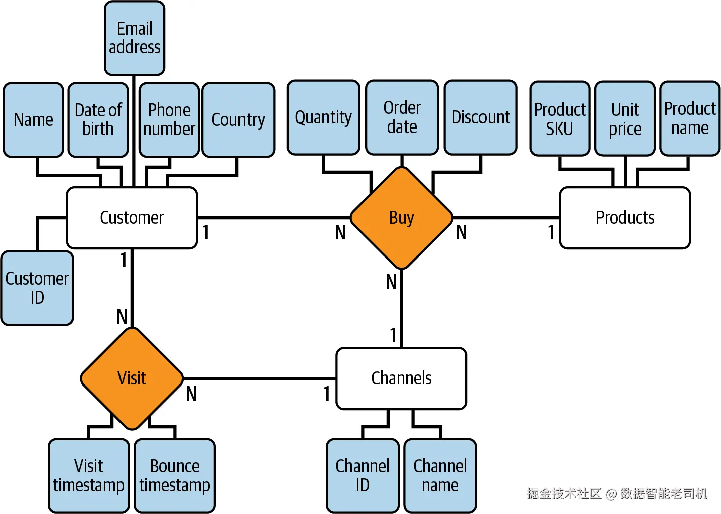
图 6-1：operational database 的 conceptual diagram

在图 6-1 的 conceptual model 中，可以看到三个 entities：Customer、Channel 和 Products，以及两个关键 relationships：Buy 和 Visit。第一个 relationship 使我们能够跟踪 customers 在特定 channels 中购买特定 products 的行为。（请记住，我们需要 channels 来理解不同 channels 的 performance。）第二个 relationship 使我们能够跟踪跨 channels 的 interactions。对于每个 entity 和 relationship，我们都定义了一些 attributes，使 database 更丰富。

Logical Model

正如前面所提到，为了将 conceptual ERD exercise 转换成 logical schema，我们会创建 entities、attributes 及其 relationships 的结构化表示。这个 schema 是在特定系统中实现 database 的基础。我们将 entities 转换为 tables，并将它们的 attributes 转换为 table columns。Relationships 会根据类型以不同方式处理：对于 N:1 relationships，我们使用 foreign keys 连接 tables；对于 M:N relationships，我们创建一张独立 table 来表示连接。通过遵循这些步骤，我们几乎会隐式地 normalize conceptual model，从而确保 data integrity 和 database 的高效管理。

如果将前面的规则应用到我们的概念模型上，应该能得到类似图 6-2 的结果。

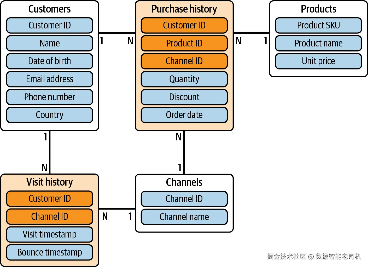
图 6-2：operational database 的 logical schema

可以看到，现在我们有五张 tables：其中三张表示 primary entities，即 Customers、Products 和 Channels；另外两张表示 relationships。不过，为了简化，我们将两张 relationship tables 分别从 Buy 和 Visit 重命名为 Purchase history 和 Visit history。

Physical Model

Logical model 主要处理 database 的 conceptual representation，而 physical model 则深入 data management 的实践层面，前提是假设我们已经选择了某个 database engine。在我们的案例中，它是 MySQL。因此，我们需要按照 MySQL 的 best practices 和 limitations，将 logical model 转换为具体的 storage configurations。

图 6-3 展示了我们的 ERD diagram，其中表示了 MySQL data types 和 constraints。

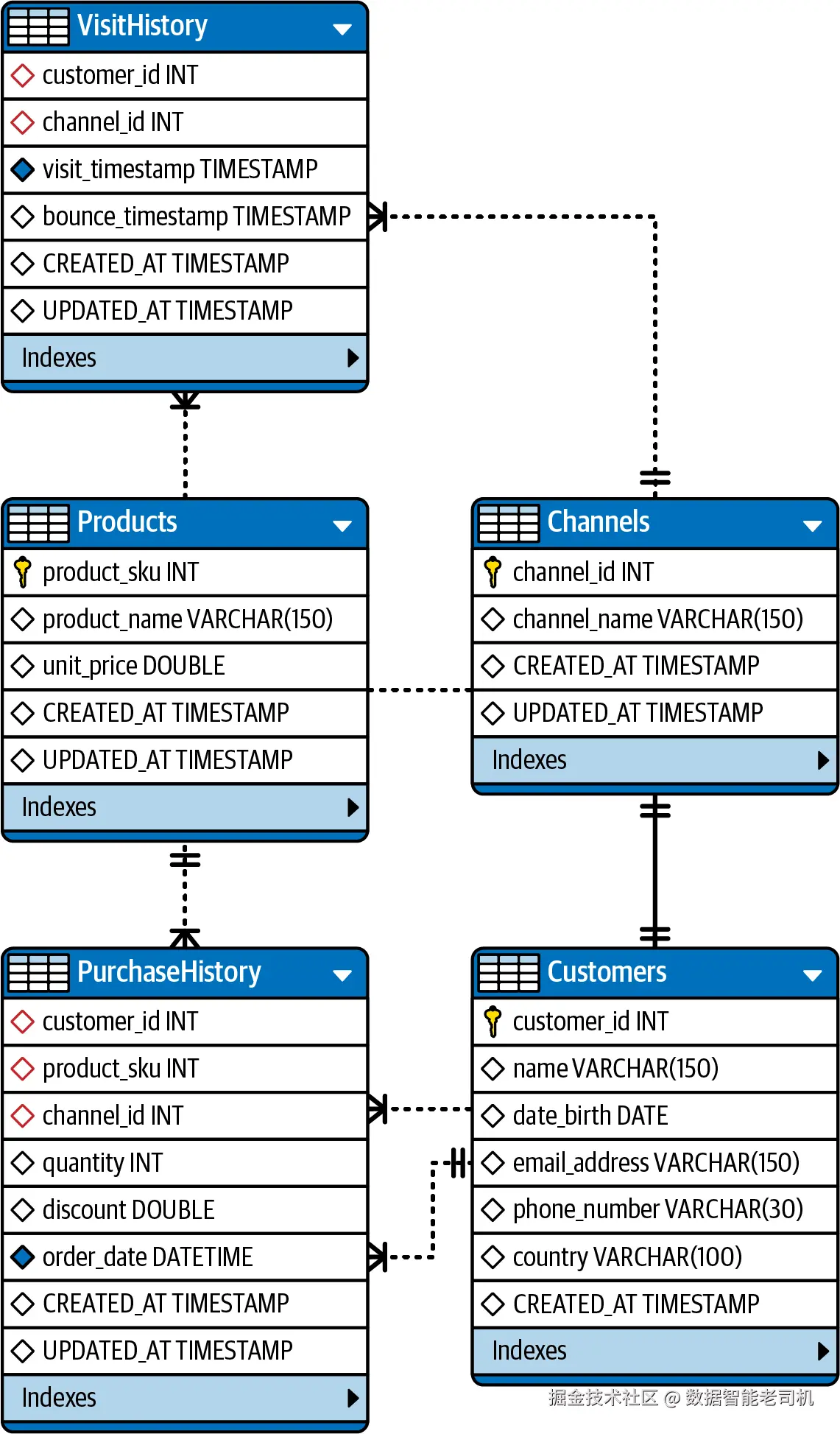
图 6-3：MySQL 中 operational database 的 physical diagram

现在，我们可以将前面的 model 转换为一组 DDL scripts，首先创建一个新的 MySQL database 来存储 table structures（Example 6-1）。

Example 6-1：Creating the primary tables

CREATE DATABASE IF NOT EXISTS OMNI_MANAGEMENT;
USE OMNI_MANAGEMENT;

在 Example 6-2 中，我们处理用于创建三张 primary tables 的 DDL code：customers、products 和 channels。

Example 6-2：Creating our operational database

CREATE TABLE IF NOT EXISTS customers (
    customer_id INT PRIMARY KEY AUTO_INCREMENT,
    name VARCHAR(150),
    date_birth DATE,
    email_address VARCHAR(150),
    phone_number VARCHAR(30),
    country VARCHAR(100),
    CREATED_AT TIMESTAMP DEFAULT CURRENT_TIMESTAMP,
    UPDATED_AT TIMESTAMP DEFAULT CURRENT_TIMESTAMP ON UPDATE CURRENT_TIMESTAMP
);

CREATE TABLE IF NOT EXISTS products (
    product_sku INTEGER PRIMARY KEY AUTO_INCREMENT,
    product_name VARCHAR(150),
    unit_price DOUBLE,
    CREATED_AT TIMESTAMP DEFAULT CURRENT_TIMESTAMP,
    UPDATED_AT TIMESTAMP DEFAULT CURRENT_TIMESTAMP ON UPDATE CURRENT_TIMESTAMP
);

CREATE TABLE IF NOT EXISTS channels (
    channel_id INTEGER PRIMARY KEY AUTO_INCREMENT,
    channel_name VARCHAR(150),
    CREATED_AT TIMESTAMP DEFAULT CURRENT_TIMESTAMP,
    UPDATED_AT TIMESTAMP DEFAULT CURRENT_TIMESTAMP ON UPDATE CURRENT_TIMESTAMP
);

customers table 包含 customer_id、name、date_birth、email_address、phone_number 和 country 等 columns。customer_id column 作为 primary key，用于唯一标识每个 customer。它被设置为每新增一个 customer 自动递增。其他 columns 存储与 customer 相关的信息。

products 和 channels tables 采用类似方式。不过，products 包含 product_sku、product_name 和 unit_price 等 columns；而 channels 只包含 channel_id 和 channel_name。

所有 tables 的创建代码中都包含 MySQL 可用的 IF NOT EXISTS clause，用于确保只有在 database 中尚不存在这些 tables 时才创建它们。这有助于在多次执行代码时避免错误或冲突。

我们在所有 tables 中都使用了 CREATED_AT 和 UPDATED_AT columns，因为这是一种 best practice。通过添加这些通常被称为 audit columns 的字段，我们让 database 为未来的数据 incremental extractions 做好准备。这也是许多 CDC tools 所要求的，因为这些工具会为我们处理这种 incremental extraction。

现在可以创建 relationship tables，如 Example 6-3 所示。

Example 6-3：Creating the relationship tables

CREATE TABLE IF NOT EXISTS purchaseHistory (
    customer_id INTEGER,
    product_sku INTEGER,
    channel_id INTEGER,
    quantity INT,
    discount DOUBLE DEFAULT 0,
    order_date DATETIME NOT NULL,
    CREATED_AT TIMESTAMP DEFAULT CURRENT_TIMESTAMP,
    UPDATED_AT TIMESTAMP DEFAULT CURRENT_TIMESTAMP ON UPDATE CURRENT_TIMESTAMP,
    FOREIGN KEY (channel_id) REFERENCES channels(channel_id),
    FOREIGN KEY (product_sku) REFERENCES products(product_sku),
    FOREIGN KEY (customer_id) REFERENCES customers(customer_id)
);

CREATE TABLE IF NOT EXISTS visitHistory (
    customer_id INTEGER,
    channel_id INTEGER,
    visit_timestamp TIMESTAMP NOT NULL,
    bounce_timestamp TIMESTAMP NULL,
    CREATED_AT TIMESTAMP DEFAULT CURRENT_TIMESTAMP,
    UPDATED_AT TIMESTAMP DEFAULT CURRENT_TIMESTAMP ON UPDATE CURRENT_TIMESTAMP,
    FOREIGN KEY (channel_id) REFERENCES channels(channel_id),
    FOREIGN KEY (customer_id) REFERENCES customers(customer_id)
);

purchaseHistory table 很可能是 purchase relationship 的核心。它包含 customer_id、product_sku、channel_id、quantity、discount 和 order_date 等 columns。customer_id、product_sku 和 channel_id columns 表示 foreign keys，分别引用 customers、products 和 channels tables 中的 primary keys。这些 foreign keys 建立了 tables 之间的 relationships。quantity column 存储所购买 products 的数量，而 discount column 保存该次 purchase 应用的 discount，默认值为 0，假设这是常规情况。order_date column 记录 purchase 的日期和时间，并被标记为 NOT NULL，意味着它必须始终有值。

visitHistory table 与 PurchaseHistory 类似，包含 customer_id、channel_id、visit_timestamp 和 bounce_timestamp 等 columns。customer_id 和 channel_id columns 作为 foreign keys，引用 customers 和 channels tables 的 primary keys。visit_timestamp column 捕获 customer 访问特定 channel 的时间戳，而 bounce_timestamp 则记录如果该次访问导致 bounce，也就是用户未进一步操作就离开 channel 时的时间戳。

FOREIGN KEY constraints 会强制 referential integrity，确保 foreign-key columns 中的 values 对应 referenced tables，即 customers、products 和 channels 中已有的 values。这有助于维护 database 内 data 的 integrity 和 consistency。

Operational database modeling 是 analyst skill set 中很有价值的一部分，即使他们并不总是直接负责设计 raw database structures。理解 operational database modeling 背后的原则和考量，可以让 analysts 对整个 data pipeline 拥有 holistic perspective。这些知识帮助他们理解自己正在处理的数据的 origin 和 structure，从而能够更有效地与负责 operational layer 的 data engineers 协作。

虽然从零设计这些 databases 并不是 analysts 和 analytics engineers 的职责，但具备 operational modeling 知识后，他们可以更好地理解 data sources 的复杂性，并确保 data 的结构和组织方式能够满足 analytical needs。此外，这种理解也有助于 troubleshooting 和 optimizing data pipelines，因为 analytics engineers 可以识别 operational database layer 中潜在问题或改进机会。本质上，熟悉 operational database modeling 可以提升 analytical skills，并促进更高效、更协作的 data-driven workflows。

High-Level Data Architecture

我们设计了一个轻量 data architecture，用于支持 omnichannel use case 的初始 requirements。我们将首先开发一个 Python script，从 MySQL 中 extract data，清洗少量 data types，然后将 data 发送到 BigQuery project。图 6-4 展示了我们的目标 solution。

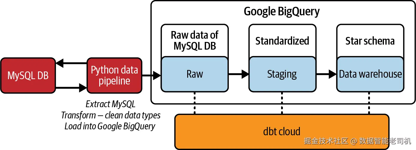
图 6-4：支持该 use case 的轻量 data architecture diagram

一旦 data 落到 raw environment，我们会利用 dbt 来 transform data，并构建构成 star schema 所需的 models。最后，我们会在 BigQuery 中针对 star schema data model 运行 SQL queries 来分析 data。

为了从 MySQL extract data 并 load 到 BigQuery，我们决定模拟一个 ETL job（Example 6-4）。Orchestrator code block 包含一个单独 function：data_pipeline_mysql_to_bq，它执行几个步骤：从 MySQL database 中 extract data、transform data，并将其 load 到 BigQuery 中的 target dataset。代码首先导入必要 modules，包括用于 MySQL database connectivity 的 mysql.connector，以及用于 data manipulation 的 pandas。另一个关键 library pandas_bq 也会在后续代码结构中使用。

data_pipeline_mysql_to_bq function 接收 keyword arguments（**kwargs），用于获取 pipeline 所需的 configuration details。在 Python 中，**kwargs 是一种特殊语法，用于将可变数量的 keyword arguments 作为类似 dictionary 的 object 传递给 function。在 function 内部，会使用提供的 connection details 与 MySQL database 建立连接。

为了自动化 table extraction，由于我们希望获取 source database 中所有 tables，因此使用 MySQL 的 information_schema 创建了一个简单 routine。information_schema 是一个 virtual database，提供对 database server、databases、tables、columns、indexes、privileges 和其他重要 metadata 的访问。它是 MySQL 自动创建并维护的 system schema。我们利用 information_schema 获取 database 中所有 table names，并将结果存储到名为 df_tables 的 DataFrame 中。

完成这一步后，我们启动 pipeline 的核心逻辑，调用 extraction、transformation 和 load functions，以模拟 ETL job 中的三个步骤。Example 6-4 中的代码片段展示了如何创建这些 functions。

Example 6-4：Loading data into BigQuery

import mysql.connector as connection
import pandas as pd

def data_pipeline_mysql_to_bq(**kwargs):

    mysql_host = kwargs.get('mysql_host')
    mysql_database = kwargs.get('mysql_database')
    mysql_user = kwargs.get('mysql_user')
    mysql_password = kwargs.get('mysql_password')
    bq_project_id = kwargs.get('bq_project_id')
    dataset = kwargs.get('dataset')

    try:
        mydb = connection.connect(host=mysql_host\
                                , database = mysql_database\
                                , user=mysql_user\
                                , passwd=mysql_password\
                                ,use_pure=True)

        all_tables = "Select table_name from information_schema.tables
                     where table_schema = '{}'".format(mysql_database)
        df_tables = pd.read_sql(all_tables,mydb,
                   parse_dates={'Date': {'format': '%Y-%m-%d'}})

        for table in df_tables.TABLE_NAME:
            table_name = table

            # Extract table data from MySQL
            df_table_data = extract_table_from_mysql(table_name, mydb)

            # Transform table data from MySQL
            df_table_data = transform_data_from_table(df_table_data)

            # Load data to BigQuery
            load_data_into_bigquery(bq_project_id,
                                  dataset,table_name,df_table_data)

            # Show confirmation message
            print("Ingested table {}".format(table_name))

        mydb.close() #close the connection
    except Exception as e:
        mydb.close()
        print(str(e))

在 Example 6-5 中，我们定义了 extract_table_from_mysql function，用来模拟 ETL job 中的 extraction step。该 function 负责从 MySQL database 中指定 table 检索 data。它接收两个 parameters：table_name 表示要 extract 的 table 名称，my_sql_connection 表示 MySQL database 的 connection object 或 connection details。

为了执行 extraction，该 function 通过把 table name 与 select * from statement 拼接来构造 SQL query。这是一种非常简单的全量抽取方式，在我们的示例中很好用。不过，在实际场景中，你可能希望通过过滤 updated_at 或 created_at 大于上次 extraction date 的 records 来进行 incremental extraction，而上次 extraction date 可以存储在 metadata table 中。

接下来，该 function 使用 pandas library 中的 pd.read_sql function 执行 extraction query。它将 query 和 MySQL connection object（my_sql_connection）作为 arguments 传入。该 function 从指定 table 读取 data，并加载到名为 df_table_data 的 pandas DataFrame 中。最后，它返回 extracted DataFrame，其中包含从 MySQL table 检索到的数据。

Example 6-5：Loading data into BigQuery---extraction

'''
    Simulate the extraction step in an ETL job
'''
def extract_table_from_mysql(table_name, my_sql_connection):
    # Extract data from mysql table
    extraction_query = 'select * from ' + table_name
    df_table_data = pd.read_sql(extraction_query,my_sql_connection)
    return df_table_data

在 Example 6-6 中，我们定义了 transform_data_from_table function，它表示 ETL job 中的 transformation step。这个 function 负责对名为 df_table_data 的 DataFrame 执行一个特定 transformation。在这个案例中，我们做了一件简单的事：清洗 DataFrame 中的 dates，将它们转换为 strings，以避免与 pandas_bq library 发生冲突。为实现这一点，该 function 使用 select_dtypes method 识别 object data type 的 columns，也就是 string columns。然后遍历这些 columns，并通过将每个 column 中的第一个 value 转换成 string representation 来检查 data type。

如果 data type 被识别为 <class datetime.date>，表示该 column 包含 date values，那么 function 会继续将每个 date value 转换为 string format。这是通过使用 lambda function 将每个 value 映射为其 string representation 完成的。执行 transformation 后，该 function 返回清洗 dates 后的 modified DataFrame。

Example 6-6：Loading data into BigQuery---transformation

'''
    Simulate the transformation step in an ETL job
'''
def transform_data_from_table(df_table_data):
    # Clean dates - convert to string
    object_cols = df_table_data.select_dtypes(include=['object']).columns
    for column in object_cols:
        dtype = str(type(df_table_data[column].values[0]))
        if dtype == "<class 'datetime.date'>":
            df_table_data[column] = df_table_data[column].map(lambda x: str(x))
    return df_table_data

在 Example 6-7 中，我们定义了 load_data_into_bigquery method，它提供一种便利方式，使用 pandas_gbq library 将 pandas DataFrame 中的数据加载到指定 BigQuery table 中。它确保 existing table 被 new data 替换，从而支持在 BigQuery environment 中进行无缝 data transfer 和 update。

该 function 接收四个 parameters：bq_project_id 表示 BigQuery project 的 project ID，dataset 和 table_name 分别指定 BigQuery 中的 target dataset 和 table。df_table_data parameter 是包含要加载数据的 pandas DataFrame。

Example 6-7：Loading data into BigQuery---load

'''
    Simulate the load step in an ETL job
'''
def load_data_into_bigquery(bq_project_id, dataset,table_name,df_table_data):
    import pandas_gbq as pdbq
    full_table_name_bg = "{}.{}".format(dataset,table_name)
    pdbq.to_gbq(df_table_data,full_table_name_bg,project_id=bq_project_id,
      if_exists='replace')

在 Example 6-8 中，我们通过使用指定 keyword arguments 调用 data_pipeline_mysql_to_bq function 来执行 data pipeline。代码创建一个名为 kwargs 的 dictionary，用来保存 function 所需的 keyword arguments。这是一种在 Python 中传递多个 parameters 的便利方式，无需将它们全部添加到 method signature 中。kwargs dictionary 包含 BigQuery project ID、dataset name、MySQL connection details（host、username、password），以及包含待传输 data 的 MySQL database 名称。不过，BigQuery project ID、MySQL host information、username 和 password 的实际 values 需要替换为合适的 values。

我们通过将 kwargs dictionary 的内容作为 keyword arguments 提供，来调用 data_pipeline_mysql_to_bq function。这会触发 data pipeline，将 data 从指定 MySQL database 移动到目标 BigQuery table。

Example 6-8：Loading data into BigQuery---call orchestrator

# Call main function

kwargs = {
    # BigQuery connection details
    'bq_project_id': <ADD_YOUR_BQ_PROJECT_ID>,
    'dataset': 'omnichannel_raw',
    # MySQL connection details
    'mysql_host': <ADD_YOUR_HOST_INFO>,
    'mysql_user': <ADD_YOUR_MYSQL_USER>,
    'mysql_password': <ADD_YOUR_MYSQL_PASSWORD>,
    'mysql_database': 'OMNI_MANAGEMENT'
}

data_pipeline_mysql_to_bq(**kwargs)

现在，raw data 应该已经加载到 BigQuery 中的 target dataset，准备使用 dbt 转换为 dimensional model。

Analytical Data Modeling

正如本书前面所见，analytical data modeling 使用一种系统化方法，包含几个关键步骤，用于创建能够有效且有意义地表示 business processes 的模型。第一步是识别并理解驱动组织运转的 business processes。这包括梳理关键 operational activities、data flows，以及 departments 之间的 interdependencies。通过充分理解 business processes，你可以准确定位 data 被 generated、transformed 和 utilized 的关键 touchpoints。

一旦你对 business processes 有了清晰认识，下一步就是在 dimensional data model 中识别 facts 和 dimensions。Facts 表示你想分析的 measurable 和 quantifiable data points，例如 sales figures、customer orders 或 website traffic。另一方面，dimensions 为这些 facts 提供必要 context。它们定义描述 facts 的各种 attributes 和 characteristics。识别这些 facts 和 dimensions 对有效 structuring data model 至关重要。

识别 facts 和 dimensions 之后，下一步是识别每个 dimension 的 attributes。Attributes 提供额外细节，并支持对 data 进行更深入分析。它们描述与每个 dimension 相关的 specific characteristics 或 properties。以 product dimension 为例，attributes 可以包括 product color、size、weight 和 price。同样，如果我们想构建 customer dimension，attributes 可能包括 demographic information，例如 age、gender 和 location。通过识别相关 attributes，可以增强 data model 的 richness 和 depth，从而支持更有洞察力的 analysis。

定义 business facts 的 granularity 是 analytical data modeling 的最后一步。Granularity 指你捕获和分析 business facts 的 detail level。必须在捕获足够细节以支持 meaningful analysis 和避免不必要 data complexity 之间取得平衡。例如，在 retail sales analysis 中，granularity 可以定义为 transaction level，捕获 individual customer purchases。另一种选择是更高层级的 granularities，例如 daily、weekly 或 monthly aggregates。Granularity 的选择取决于 analytical objectives、data availability，以及推导 valuable insights 所需的 detail level。

通过遵循这些 analytical data modeling 步骤，你可以建立一个坚实基础，创建准确表示 business、捕获 essential facts 和 dimensions、包含 relevant attributes，并定义适当 granularity level 的 data model。设计良好的 data model 使你能够释放 data 的力量，获得 valuable insights，并做出 informed decisions，从而推动 business growth 和 success。

Identify the Business Processes

在开发有效 analytical data model 的过程中，初始阶段是识别组织中的 business processes。在与 key stakeholders 讨论并进行深入 interviews 后，我们发现主要 objectives 之一，是跨 channels 跟踪 sales performance。这一关键信息将为 revenue generation 和各种 sales channels 的 effectiveness 提供 valuable insights。

进一步探索组织目标时，还发现另一个重要 requirement：按 channel 跟踪 visits 和 bounce rates。这个目标旨在揭示跨 channels 的 customer engagement 和 website performance。通过衡量 visits 数量和 bounce rates，组织可以识别哪些 channels 正在带来 traffic，以及哪些方面需要改进，以减少 bounce rates 并提升 user engagement。

理解这些 metrics 的重要性后，我们意识到需要关注两个不同的 business processes：sales tracking 和 website performance analysis。Sales tracking process 会捕获并分析通过各种 channels 产生的 sales data，例如 mobile、mobile app 或 Instagram。该过程将提供 sales performance 的全面视图，使组织能够围绕 channel optimization 和 sales forecasting 做出 data-driven decisions。

与此同时，website performance analysis process 会收集各种 channels 上的 website visits 和 bounce rates 数据。这需要实现 robust tracking mechanisms，例如 web analytics tools，用于监控和衡量用户在组织网站上的行为。通过检查 channel-specific visit patterns 和 bounce rates，组织可以识别 trends、优化 user experience，并提升 website performance，以改进整体 customer engagement。

因此，识别这两个关键 business processes------sales tracking 和 website performance analysis------成为 analytical data modeling 旅程中的一个重要里程碑。有了这些知识，我们就具备了进入下一阶段的条件。在下一阶段，我们将更深入理解与这些 processes 相关的 data flows、interdependencies 和 specific data points，塑造一个与组织 objectives 和 requirements 对齐的 comprehensive dimensional data model。

Identify Facts and Dimensions in the Dimensional Data Model

基于已识别的 sales tracking 和 website performance analysis 两个 business processes，我们推断需要四个 dimensions 和两个对应 fact tables。下面逐一说明。

第一个 dimension 是 channels（dim_channels）。该 dimension 表示组织运营所涉及的各种 sales 和 marketing channels。识别出的常见 channels 包括 website、Instagram 和 mobile app channels。通过分析 across channels 的 sales data，组织可以获得每个 channel 在 revenue generation 方面的 performance 和 effectiveness insights。

第二个 dimension 是 products（dim_products）。该 dimension 聚焦组织的 product offerings。通过包含 product dimension，组织能够分析不同 product categories 的 sales patterns，并识别 top-selling products 或需要改进的 areas。

第三个 dimension 是 customers（dim_customers）。该 dimension 捕获组织 customer base 的相关信息。通过基于 customer attributes 分析 sales data，组织可以获得 customer preferences、behavior 和 purchasing patterns 方面的 insights。

第四个也是最后一个 dimension 是 date（dim_date）。该 dimension 允许按时间分析 sales 和 website performance。基于 date dimension 分析 data，使组织能够识别 trends、seasonality，以及可能影响 sales 或 website performance 的 temporal patterns。

现在进入 fact tables。识别出的第一张 fact table 是 purchase history（fct_purchase_history）。这张 table 作为中心点，捕获 purchase transactions，并将其与相关 dimensions 关联起来：channels、products、customers 和 date。它支持详细的 sales data analysis，使组织能够理解 sales 与各 dimensions 之间的 correlation。通过 purchase history fact table，组织可以获得 across channels、product categories、customer segments 和 time periods 的 sales performance insights。

第二张 fact table 是 visits history table（fct_visit_history）。不同于 purchase history，这张 table 聚焦 website performance analysis。它捕获与 website visits 相关的数据，并主要与 channels、customers 和 date dimensions 关联。通过分析 visit history，组织可以理解 customer engagement，跟踪 across channels 的 traffic patterns，并衡量不同 marketing campaigns 或 website features 的 effectiveness。

识别出这些 dimensions 和 fact tables 后，我们已经为 dimensional data model 奠定了基础。这个 model 使你能够高效分析并从 various dimensions 下的 sales data 中推导 insights，同时跟踪与不同 channels、customers 和 time periods 相关的网站 performance metrics。随着 data modeling process 推进，我们将进一步细化并定义每个 dimension 中的 attributes，并建立 comprehensive analysis 所需的 relationships 和 hierarchies。但目前，我们已经具备设计 star schema 的条件（图 6-5）。

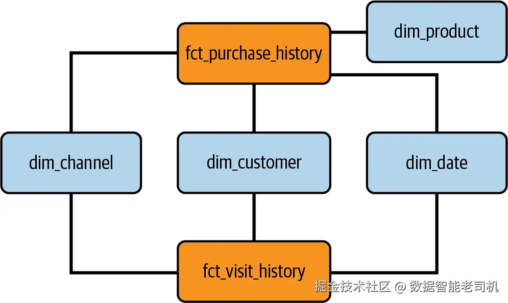
图 6-5：Use case star schema model

Star schema 包含四个 primary dimensions：channels、products、customers 和 date。这些 dimensions 是分析的支柱，为 data 提供有价值的 context。

NOTE

其中三个 dimensions，即 dim_channels、dim_customers 和 dim_date，是 conformed dimensions。Conformed dimensions 会在多个 fact tables 之间共享，确保 consistency，并促进不同 analytical perspectives 之间的无缝集成。

Identify the Attributes for Dimensions

识别出 dimensions 后，就到了详细定义每个 dimension 中 identified attributes 的时候。通过将这些 attributes 纳入对应 dimensions，data model 会获得更深度和完整性。这些 attributes 丰富了 analysis，并支持更 granular insights，使 decision-makers 能够从 data 中推导 valuable information。

对于 channels dimension（dim_channels），识别出多个 attributes。首先，channel surrogate key（sk_channel）为 data model 中每个 channel 提供 unique identifier。与它配套的是 channel natural key（nk_channel_id），它表示来自 source system 的 key，确保与 external data sources 的 seamless integration。此外，channel name attribute（dsc_channel_name）捕获每个 channel 的 descriptive name，使其在 data model 中易于识别和理解。最后这个 attribute 对 analytics 来说可能最有价值。

进入 products dimension（dim_products），识别出多个关键 attributes。Product surrogate key（sk_product）作为 data model 中每个 product 的 unique identifier。类似地，product natural key（nk_product_sku）捕获来自 source system 的 key，支持 product-related data 的一致连接。Product name attribute（dsc_product_name）提供每个 product 的 descriptive name，有助于 clarity 和 comprehension。最后，product unit price attribute（mtr_unit_price）记录每个 product 的 price，便于 price analysis 和 revenue calculations。

在 customers dimension（dim_customers）中，不同 attributes 有助于提供 customer-related information 的全面视图。Customer surrogate key（sk_customer）是 data model 中每个 customer 的 unique identifier。Customer natural key（nk_customer_id）保留来自 source system 的 key，支持与 external data sources 的无缝集成。此外，customer name（dsc_name）、birth date（dt_date_birth）、email address（dsc_email_address）、phone number（dsc_phone_number）和 country（dsc_country）等 attributes 捕获与 individual customers 相关的重要 details。这些 attributes 支持 customer segmentation、personalized marketing，以及深入的 customer behavior 和 demographics analysis。

最后，date dimension（dim_date）包含一系列 date-related attributes。这些 attributes 增强了对 temporal data 的理解和分析。Date attribute 本身捕获具体日期。Month、quarter 和 year 等 attributes 提供更高层级的 temporal information，便于 aggregated analysis。通过包含这些 attributes，data model 支持全面的 time-based analysis 和 pattern recognition。

TIP

Surrogate keys 是分配给 database table 中 records 的人工 identifiers。它们为 data operations 提供 uniqueness、stability 和 improved performance。Surrogate keys 独立于 data 本身，确保每条 record 都有唯一 identifier，并且即使 natural key values 发生变化，也能保持稳定。它们简化 tables 之间的 joins，增强 data integration，并促进高效 indexing 和 querying。

Define the Granularity for Business Facts

完成 analytical data modeling 的前面阶段后，现在进入最后一个关键步骤，也就是识别未来 business facts 的 granularity。Granularity 指在 dimensional data model 中捕获和分析 data 的 detail level。确定合适 granularity 对确保 data model 能有效支持组织的 analytical requirements 和 objectives 至关重要。

为了定义 business facts 的 granularity，需要考虑 analysis 的具体需求，并在捕获足够细节和避免过度 complexity 之间取得平衡。选择的 granularity 应提供足够信息来支持 meaningful analysis，同时保持 data manageability 和 performance。

在 sales data context 中，识别出的 granularity 被确定为 transaction level，用于捕获 individual customer purchases：fct_purchase_history。这个 granularity level 支持对 sales patterns 的详细分析，例如检查 individual transactions、识别 customer behavior trends，并进行 product-level analysis。

对于另一个 requirement，即 website performance analysis，granularity 被选择为 visit level，收集 individual customer visits 及其进入 platform 的 channel：fct_visit_history。有了这种细节，组织可以理解 customer engagement，跟踪 across channels 的 traffic patterns，并衡量不同 marketing campaigns 或 website features 的 effectiveness。

或者，在定义好 granularities 后，也可以确定更低粒度的其他 analysis units，例如 daily、weekly 或 monthly aggregates。Aggregating data 可以在提供 valuable insights 的同时，以更简洁的方式表示 data。这种 approach 减少 data volume，并简化 analysis，使识别 broader trends、seasonal patterns 或跨多个 dimensions 的整体 performance 更容易。

通过仔细定义 business facts 的 granularity，组织可以确保 dimensional data model 在捕获足够细节与保持 data manageability 和 performance 之间达到正确平衡。这一步为 meaningful analysis 奠定基础，使 stakeholders 能够基于 data 推导 valuable insights 并做出 informed decisions。

随着本阶段结束，我们已经成功走过 analytical data modeling 的关键阶段，包括识别 business processes、facts、dimensions 和 attributes，以及定义 business facts 的 granularity。这些基础步骤为开发全面且有效的 dimensional data model 提供了坚实框架，使组织能够进行 data-driven decision making。下一节中，我们将动手使用 dbt 开发 models，但始终基于 analytical data modeling 所定义的基础。

Creating Our Data Warehouse with dbt

Analytical data modeling 阶段完成后，是时候进入 data warehouse 开发了。Data warehouse 是 structured 和 integrated data 的中心 repository，支持组织内部 robust reporting、analysis 和 decision-making processes。

总体上，data warehouse development 从建立必要 infrastructure 开始。简单来说，我们之前已经在 "High-Level Data Architecture" 中完成了这一步，也就是设置 BigQuery。到了这个阶段，只需要设置 dbt project，并将其连接到 BigQuery 和 GitHub。在 "Setting Up dbt Cloud with BigQuery and GitHub" 中，我们已经提供了完整 step-by-step guide，解释如何完成所有 initial setup，因此本节会跳过这个阶段。

本节的主要目标，是开发 analytical data modeling 阶段中设计好的全部 dbt models。它们是 data warehouse 设计和构建的 blueprint。在开发 models 的同时，我们还会开发所有 parametrization YAML files，以确保使用 ref() 和 source() functions，并最终让代码更 DRY。与上述目标一致，在开发 YAML files 的同时，还需要执行另一个步骤：构建 staging models area。这些 models 将成为 dimensions 和 facts 的种子。

除了开发 data models，还必须在 data warehouse 内建立一致的 naming conventions。这些 naming conventions 为 tables、columns 和其他 database objects 的命名提供标准化方法，确保整个 data infrastructure 具备 clarity 和 consistency。表 6-1 展示了使用 dbt 构建 data warehouse 时采用的 naming conventions。

表 6-1：Naming conventions

Convention	Field type	Description
stg	Table/CTE	Staging tables or CTE
dim	Table	Dimension tables
fct	Table	Fact tables
nk	Column	Natural keys
sk	Column	Surrogate keys
mtr	Column	Metric columns（numeric values）
dsc	Column	Description columns（text values）
dt	Column	Date and time columns

为了构建第一个 models，必须确保 dbt project 已经设置完成，并且拥有正确 folder structure。在 use case 的这一部分，我们会保持简单，只构建 staging 和 marts directories。因此，一旦初始化好 dbt project，就创建指定 folders。Models folder directory 应该类似 Example 6-9。

Example 6-9：Omnichannel data warehouse，models directory

root/
├─ models/
│  ├─ staging/
│  ├─ marts/
├─ dbt_project.yml

现在我们已经建立了初始 project 和 folders，下一步是创建 staging YAML files。根据 "YAML Files" 中讨论的 YAML files segregation best practices，我们会为 sources 创建一个 YAML file，再为 models 创建另一个 YAML file。为了构建 staging layer，暂时只关注 source YAML file。这个 file 必须位于 staging directory 中，内容应类似 Example 6-10。

Example 6-10：_omnichannel_raw_sources.yml file configuration

version: 2

sources:
  - name: omnichannel
    database: analytics-engineering-book
    schema: omnichannel_raw
    tables:
      - name: Channels
      - name: Customers
      - name: Products
      - name: VisitHistory
      - name: PurchaseHistory

使用这个 file 后，你就可以利用 source() function 来处理 data platform 中可用的 raw data。在 omnichannel_raw schema 下指定了五张 tables：Channels、Customers、Products、VisitHistory 和 PurchaseHistory。它们对应于构建 staging layer 所需的相关 source tables，dbt 会与这些 tables 交互来构建 staging data models。

让我们开始构建 staging models。这里的核心思路是，为每个 source table 创建一个 staging model：Channels、Customers、Products、VisitHistory 和 PurchaseHistory。请记住，每个新的 staging model 都需要创建在 staging directory 内。

Examples 6-11 到 6-15 展示了构建每个 staging model 的代码片段。

Example 6-11：stg_channels

with raw_channels AS
(
    SELECT
        channel_id,
        channel_name,
        CREATED_AT,
        UPDATED_AT
    FROM {{ source("omnichannel","Channels")}}
)

SELECT
    *
FROM raw_channels

Example 6-12：stg_customers

with raw_customers AS
(
    SELECT
        customer_id,
        name,
        date_birth,
        email_address,
        phone_number,
        country,
        CREATED_AT,
        UPDATED_AT
    FROM {{ source("omnichannel","Customers")}}
)

SELECT
    *
FROM raw_customers

Example 6-13：stg_products

with raw_products AS
(
    SELECT
        product_sku,
        product_name,
        unit_price,
        CREATED_AT,
        UPDATED_AT
    FROM {{ source("omnichannel","Products")}}
)

SELECT
    *
FROM raw_products

Example 6-14：stg_purchase_history

with raw_purchase_history AS
(
    SELECT
        customer_id,
        product_sku,
        channel_id,
        quantity,
        discount,
        order_date
    FROM {{ source("omnichannel","PurchaseHistory")}}
)

SELECT
    *
FROM raw_purchase_history

Example 6-15：stg_visit_history

with raw_visit_history AS
(
    SELECT
        customer_id,
        channel_id,
        visit_timestamp,
        bounce_timestamp,
        created_at,
        updated_at
    FROM {{ source("omnichannel","VisitHistory")}}
)

SELECT
    *
FROM raw_visit_history

总结来说，这些 dbt models 中的每一个都会从相应 source tables 中 extract data，并将其 stage 到单独 CTEs 中。这些 staging tables 是后续 data transformations 的 intermediate storage，在 data 加载到 data warehouse 的最终 destination tables 之前使用。

成功创建 staging models 后，下一阶段是为 staging layer 设置 YAML file。Staging layer YAML file 将作为 configuration file，引用 staging models，并指定它们的 execution order 和 dependencies。这个 file 为 staging layer 的 setup 提供了清晰且结构化的视图，使 staging models 能够在整体 data modeling process 中一致地集成和管理。Example 6-16 展示了 staging layer 中 YAML file 应该是什么样子。

Example 6-16：_omnichannel_raw_models.yml file configuration

version: 2

models:
  - name: stg_customers
  - name: stg_channels
  - name: stg_products
  - name: stg_purchase_history
  - name: stg_visit_history

Staging layer YAML file 就位后，就可以继续构建 dimension models。Dimension models 是 data warehouse 的关键组成部分，用于表示 business entities 及其 attributes。这些 models 捕获 descriptive information，为 fact data 提供 context，并支持更深入 analysis。Dimension tables，例如 channels、products、customers 和 date，将基于先前定义的 dimensions 及其 attributes 构建，这些内容来自 "Identify Facts and Dimensions in the Dimensional Data Model" 和 "Identify the Attributes for Dimensions"。这些 tables 会由 staging layer 中的相关 data 填充，以确保 consistency 和 accuracy。

现在继续创建 dimension models。请在 marts directory 中创建 Examples 6-17 到 6-20 中对应的 models。

Example 6-17：dim_channels

with stg_dim_channels AS
(
    SELECT
        channel_id AS nk_channel_id,
        channel_name AS dsc_channel_name,
        created_at AS dt_created_at,
        updated_at AS dt_updated_at
    FROM {{ ref("stg_channels")}}
)

SELECT
    {{ dbt_utils.generate_surrogate_key( ["nk_channel_id"] )}} AS sk_channel,
    *
FROM stg_dim_channels

Example 6-18：dim_customers

with stg_dim_customers AS
(
    SELECT
        customer_id AS nk_customer_id,
        name AS dsc_name,
        date_birth AS dt_date_birth,
        email_address AS dsc_email_address,
        phone_number AS dsc_phone_number,
        country AS dsc_country,
        created_at AS dt_created_at,
        updated_at AS dt_updated_at
    FROM {{ ref("stg_customers")}}
)

SELECT
    {{ dbt_utils.generate_surrogate_key( ["nk_customer_id"] )}} AS sk_customer,
    *
FROM stg_dim_customers

Example 6-19：dim_products

with stg_dim_products AS
(
    SELECT
        product_sku AS nk_product_sku,
        product_name AS dsc_product_name,
        unit_price AS mtr_unit_price,
        created_at AS dt_created_at,
        updated_at AS dt_updated_at
    FROM {{ ref("stg_products")}}
)

SELECT
    {{ dbt_utils.generate_surrogate_key( ["nk_product_sku"] )}} AS sk_product,
    *
FROM stg_dim_products

Example 6-20：dim_date

{{ dbt_date.get_date_dimension("2022-01-01", "2024-12-31") }}

总结来说，每个 code block 都定义了一个特定 dimension table 的 dbt model。前三个 models，即 dim_channels、dim_customers 和 dim_products，会从对应 staging tables 检索 data，并将其转换为 dimension tables 所需的结构。在每一个 model 中，我们都包含了基于 natural key 生成 surrogate keys 的逻辑。为此，我们使用了 dbt_utils package，具体来说是 generate_surrogate_key() function。该 function 接收一个 column names 数组作为 argument，这些 columns 表示 dimension table 的 natural keys 或 business keys，并基于这些 columns 生成 surrogate key column。

最后一个 dimension，即 dim_date，则不同，因为它并不是来自 staging layer。相反，它完全使用 dbt_date package 中的 get_date_dimension() function 生成。get_date_dimension() function 会处理 date dimension table 的生成，包括基于指定 date range 创建所有必要 columns 及其数据。在我们的案例中，选择的 date range 是 2022-01-01 到 2024-12-31。

最后，请记住现在我们正在使用 packages。为了在这个阶段成功构建 project，需要安装它们。因此，将 Example 6-21 的 configurations 添加到 dbt_packages.yml file 中。然后执行 dbt deps 和 dbt build commands，并查看 data platform，检查新的 dimensions 是否已经创建。

Example 6-21：packages.yml file configuration

packages:
  - package: dbt-labs/dbt_utils
    version: 1.1.1
  - package: calogica/dbt_date
    version: [">=0.7.0", "<0.8.0"]

最后一步是创建 fact tables 对应的 models，这些 fact tables 是前面识别出的、用于分析新 business processes 所必需的表。它们是 data warehouse 的重要组成部分，表示捕获 business events 或 transactions 的 measurable、numerical data。

Examples 6-22 和 6-23 表示要开发的新 fact tables。请在 marts directory 中创建它们。

Example 6-22：fct_purchase_history

with stg_fct_purchase_history AS
(
    SELECT
        customer_id AS nk_customer_id,
        product_sku AS nk_product_sku,
        channel_id AS nk_channel_id,
        quantity AS mtr_quantity,
        discount AS mtr_discount,
        CAST(order_date AS DATE) AS dt_order_date
    FROM {{ ref("stg_purchase_history")}}
)

SELECT
    COALESCE(dcust.sk_customer, '-1') AS sk_customer,
    COALESCE(dchan.sk_channel, '-1') AS sk_channel,
    COALESCE(dprod.sk_product, '-1') AS sk_product,
    fct.dt_order_date AS sk_order_date,
    fct.mtr_quantity,
    fct.mtr_discount,
    dprod.mtr_unit_price,
    ROUND(fct.mtr_quantity * dprod.mtr_unit_price,2) AS mtr_total_amount_gross,
    ROUND(fct.mtr_quantity *
              dprod.mtr_unit_price *
              (1 - fct.mtr_discount),2) AS mtr_total_amount_net
FROM stg_fct_purchase_history AS fct
LEFT JOIN {{ ref("dim_customers")}} AS dcust
                       ON fct.nk_customer_id = dcust.nk_customer_id
LEFT JOIN {{ ref("dim_channels")}} AS dchan
                       ON fct.nk_channel_id = dchan.nk_channel_id
LEFT JOIN {{ ref("dim_products")}} AS dprod
                       ON fct.nk_product_sku = dprod.nk_product_sku

fct_purchase_history 旨在回答第一个已识别的 business process，也就是跨 channels 跟踪 sales performance。接下来，我们从 stg_purchase_history model 收集 sales data，并将其与相应 channel、customer 和 product dimensions join，以捕获对应 surrogate key，同时使用 COALESCE() function 处理 natural key 没有匹配到 dimension table entry 的情况。通过包含这个 fact 与相应 dimensions 之间的 relationship，组织将能够获得关于 revenue generation，以及不同 sales channels 在 customer 和 product 维度下 effectiveness 的 valuable insights。

为了完全满足 requirements，我们还基于所购产品数量（mtr_quantity）、每件产品的 unit price（mtr_unit_price）以及应用的 discount（mtr_discount），计算两个额外 metrics：mtr_total_amount_gross 和 mtr_total_amount_net。

总结来说，Example 6-22 展示了将 staging data 转换为结构化 fact table 的过程，该 fact table 捕获相关 purchase history information。通过 join dimension tables 并执行 calculations，fact table 提供了 purchase data 的 consolidated view，从而支持 valuable insights 和 analysis。

进入最后一张 fact table，来看 Example 6-23。

Example 6-23：fct_visit_history

with stg_fct_visit_history AS
(
    SELECT
        customer_id AS nk_customer_id,
        channel_id AS nk_channel_id,
        CAST(visit_timestamp AS DATE) AS sk_date_visit,
        CAST(bounce_timestamp AS DATE) AS sk_date_bounce,
        CAST(visit_timestamp AS DATETIME) AS dt_visit_timestamp,
        CAST(bounce_timestamp AS DATETIME) AS dt_bounce_timestamp
    FROM {{ ref("stg_visit_history")}}
)

SELECT
    COALESCE(dcust.sk_customer, '-1') AS sk_customer,
    COALESCE(dchan.sk_channel, '-1') AS sk_channel,
    fct.sk_date_visit,
    fct.sk_date_bounce,
    fct.dt_visit_timestamp,
    fct.dt_bounce_timestamp,
    DATE_DIFF(dt_bounce_timestamp,dt_visit_timestamp
                , MINUTE) AS mtr_length_of_stay_minutes
FROM stg_fct_visit_history AS fct
LEFT JOIN {{ ref("dim_customers")}} AS dcust
                   ON fct.nk_customer_id = dcust.nk_customer_id
LEFT JOIN {{ ref("dim_channels")}} AS dchan
                   ON fct.nk_channel_id = dchan.nk_channel_id

fct_visit_history 回答另一个已识别的 business process：按 channel 跟踪 visits 和 bounce rates，以揭示 across channels 的 customer engagement 和 website performance。为了创建它，我们从 stg_visit_history model 收集 visit data，并将其与 customers 和 channels dimensions join，以捕获对应 surrogate key，同时使用 COALESCE() function 处理 natural key 没有匹配到 dimension table entry 的情况。建立这个 fact 与 dimensions 的 relationship 后，组织将能够识别哪些 channels 正在带来更多 traffic。我们还添加了一个额外 calculated metric：mtr_length_of_stay_minutes，用于理解某次 visit 的 length of stay。这个 calculated metric 利用 DATE_DIFF() function 计算 bounce date 与 visit date 之间的差异，目标是支持组织识别改进 areas，以减少 bounce rates 并提升 user engagement。

总之，fct_visit_history fact table 将 staging data 转换为结构化 fact table，捕获 relevant visit history information。通过 join dimension tables 并执行 calculations，就像两个 facts 中所做的那样，fct_visit_history table 提供了 visit data 的 compact view，支持 valuable insights 和 analysis。

下一节中，我们将继续旅程，开发 tests 和 documentation，并最终部署到 production。这些将是 dbt 内部的最后步骤，目标是保证 data model 的 reliability、usability、ongoing availability，并支持组织内的 data-driven decision making。

Tests, Documentation, and Deployment with dbt

随着 data warehouse 开发接近完成，确保已实现 data models 的 accuracy、reliability 和 usability 至关重要。本节聚焦 testing、documentation，以及让 data warehouse go live。

正如前面所说，使用 dbt 时，tests 和 documentation 应该在开发 models 的同时创建。我们采取了这种 approach，但为了 clarity，将其拆成两个部分。这种划分使我们能够更清晰理解在 dbt 中完成了哪些 model development 工作，以及 testing 和 documentation processes 是如何进行的。

简单总结一下，testing 对验证 data model 的 functionality 和 integrity 至关重要。Testing 会验证 dimension 和 fact tables 之间的 relationships，检查 data consistency，并验证 calculated metrics 的 accuracy。通过执行 tests，你可以识别并纠正 data 中的任何 issues 或 discrepancies，从而确保 analytical outputs 的 reliability。

执行 singular 和 generic tests 都很重要。Singular tests 面向 data models 的特定方面，例如验证某个 specific metric calculation 的 accuracy，或验证某个 particular dimension 和 fact table 之间的 relationship。这些 tests 能对 data models 的 individual components 提供 focused insights。

另一方面，generic tests 覆盖更广泛的 scenarios，并监控 data models 的整体 behavior。这些 tests 旨在确保 data models 在不同 dimensions、time periods 和 user interactions 下都能正确运行。Generic tests 有助于发现 real-world usage 中可能出现的潜在问题，并增强对 data models 处理 various scenarios 能力的信心。

与此同时，记录 data models 和相关 processes 对 knowledge transfer、collaboration 和 future maintenance 是必要的。Documenting data models 涉及捕获关于 models 的 purpose、structure、relationships 和 underlying assumptions 的信息。它包括 source systems、transformation logic、applied business rules 以及其他相关信息的 details。

为了记录 data models，建议使用 comprehensive explanations 和 metadata 更新对应 YAML files。YAML files 是 dbt models 的 configuration 和 documentation 的集中位置，使 tracking changes 以及理解每个 model 的 purpose 和 usage 更容易。记录 YAML files 可以确保未来 team members 和 stakeholders 清楚理解 data models，并能有效使用它们。

Testing 和 documentation 完成后，本节的最后一步是准备 data warehouse 的 go-live。这包括将 data models 部署到 production environment，确保 data pipelines 已建立，并设置 scheduled data updates。在这个阶段，监控 data warehouse 的 performance、availability 和 data quality 非常重要。在 production-like environment 中进行全面 testing，并获取 end-user feedback，可以帮助在 data warehouse 完全投入运行前识别剩余问题。

让我们从 tests 开始。第一批 tests 将聚焦 generic tests。第一个 use case 是确保所有 dimensions 的 surrogate key 都是 unique 且没有 null values。第二个 use case 是必须确保 fact table 中的每个 surrogate key 都存在于指定 dimension 中。首先，在 marts layer 中创建相应 YAML file，使用 Example 6-24 的代码块来实现上述内容。

Example 6-24：_omnichannel_marts.yml file configuration

version: 2

models:
  - name: dim_customers
    columns:
      - name: sk_customer
        tests:
          - unique
          - not_null

  - name: dim_channels
    columns:
      - name: sk_channel
        tests:
          - unique
          - not_null

  - name: dim_date
    columns:
      - name: date_day
        tests:
          - unique
          - not_null

  - name: dim_products
    columns:
      - name: sk_product
        tests:
          - unique
          - not_null

  - name: fct_purchase_history
    columns:
      - name: sk_customer
        tests:
          - relationships:
              to: ref('dim_customers')
              field: sk_customer
      - name: sk_channel
        tests:
          - relationships:
              to: ref('dim_channels')
              field: sk_channel
      - name: sk_product
        tests:
          - relationships:
              to: ref('dim_products')
              field: sk_product

  - name: fct_visit_history
    columns:
      - name: sk_customer
        tests:
          - relationships:
              to: ref('dim_customers')
              field: sk_customer
      - name: sk_channel
        tests:
          - relationships:
              to: ref('dim_channels')
              field: sk_channel

现在执行 dbt test command，查看所有 tests 是否成功执行。如果 logs 如图 6-6 所示，就说明一切顺利。

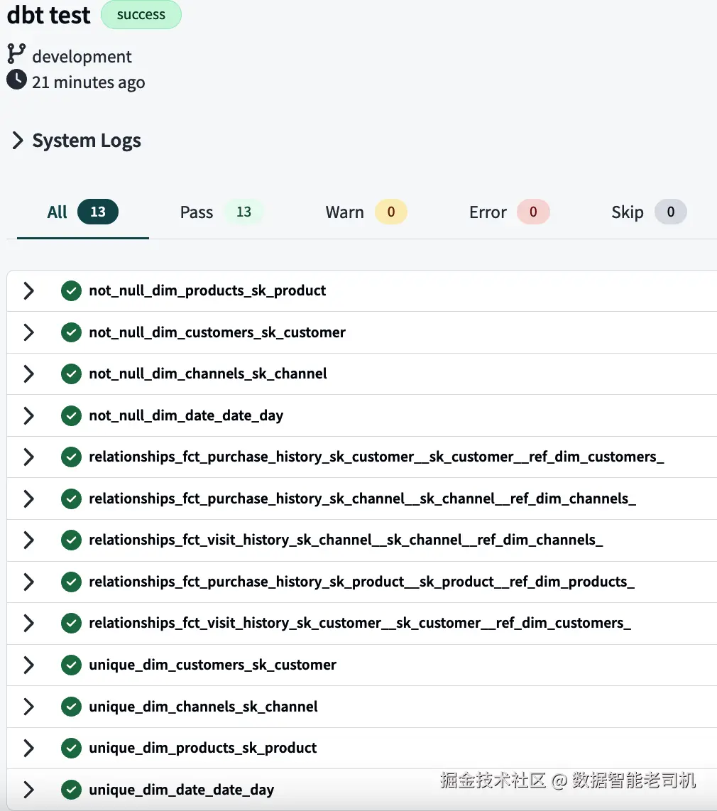
图 6-6：Generic tests 的 logs

现在进入第二轮 tests，开发一些 singular tests。这里我们聚焦 fact table metrics。第一个 singular use case 是确保 fct_purchase_history 中的 mtr_total_amount_gross metric 只有正值。为此，在 tests folder 中创建一个新 test：assert_mtr_total_amount_gross_is_positive.sql，并使用 Example 6-25 中的代码。

Example 6-25：assert_mtr_total_amount_gross_is_positive.sql

select
    sk_customer,
    sk_channel,
    sk_product,
    sum(mtr_total_amount_gross) as mtr_total_amount_gross
from {{ ref('fct_purchase_history') }}
group by 1, 2, 3
having mtr_total_amount_gross < 0

下一个 test 是确认 mtr_unit_price 始终小于或等于 mtr_total_amount_gross。注意，同样的 test 不能应用到 mtr_total_amount_net，因为它还应用了 discount。要开发这个 test，首先创建文件 assert_mtr_unit_price_is_equal_or_lower_than_mtr_total_amount_gross.sql，并粘贴 Example 6-26 中的代码。

Example 6-26：assert_mtr_unit_price_is_equal_or_lower_than_mtr_total_amount_gross.sql

select
    sk_customer,
    sk_channel,
    sk_product,
    sum(mtr_total_amount_gross) AS mtr_total_amount_gross,
    sum(mtr_unit_price) AS mtr_unit_price
from {{ ref('fct_purchase_history') }}
group by 1, 2, 3
having mtr_unit_price > mtr_total_amount_gross

所有 singular tests 创建完成后，就可以执行它们并检查 output。为了避免执行所有 tests，包括 generic tests，请执行 dbt test --select test_type:singular command。该 command 会执行 singular 类型的 tests，并忽略 generic tests。图 6-7 展示了预期 log output。

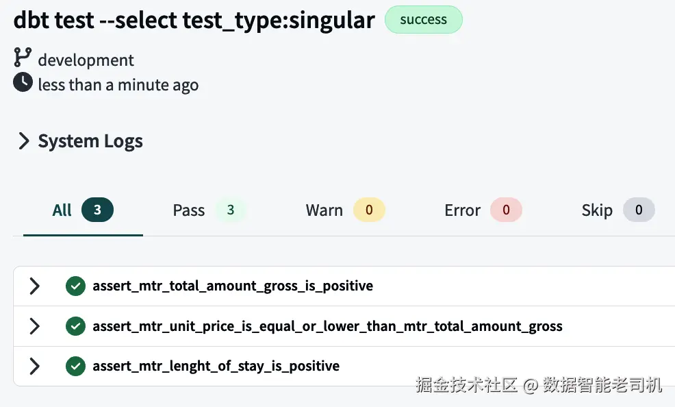
图 6-7：Singular tests 的 logs

最后一个 singular test 是确认在 fct_visit_history 中，mtr_length_of_stay_minutes metric 始终为正。这个 test 会告诉我们是否存在 bounce date 早于 visit date 的 records，而这种情况永远不应该发生。为执行它，创建 assert_mtr_length_of_stay_is_positive.sql file，并使用 Example 6-27 中的代码。

Example 6-27：assert_mtr_length_of_stay_is_positive.sql

select
    sk_customer,
    sk_channel,
    sum(mtr_length_of_stay_minutes) as mtr_length_of_stay_minutes
from {{ ref('fct_visit_history') }}
group by 1, 2
having mtr_length_of_stay_minutes < 0

通过实现 tests，你可以验证 data 的 integrity，验证 calculations 和 transformations，并确保遵守 defined business rules。dbt 提供完整 testing framework，使你能够执行 singular 和 generic tests，覆盖 data models 的多个方面。

所有 tests 成功执行后，我们进入 data warehouse development process 的下一个关键方面：documentation。在 dbt 中，documentation 的很大一部分使用与配置 models 或执行 tests 相同的 YAML files 完成。让我们使用 marts layer 记录所有 tables 和 columns。参考 _omnichannel_marts.yml file，并用 Example 6-28 中的代码替换它。需要说明的是，为了让示例更清晰，我们只记录 generic tests 中使用的 columns，但同样前提适用于其他所有 columns。

Example 6-28：带 documentation 的 _omnichannel_marts.yml file configuration

version: 2

models:
  - name: dim_customers
    description: All customers' details. Includes anonymous users who used guest
    checkout.
    columns:
      - name: sk_customer
        description: Surrogate key of the customer dimension.
        tests:
          - unique
          - not_null

  - name: dim_channels
    description: Channels data. Allows you to analyze linked facts from the channels
    perspective.
    columns:
      - name: sk_channel
        description: Surrogate key of the channel dimension.
        tests:
          - unique
          - not_null

  - name: dim_date
    description: Date data. Allows you to analyze linked facts from the date
    perspective.
    columns:
      - name: date_day
        description: Surrogate key of the date dimension. The naming convention
        wasn't added here.
        tests:
          - unique
          - not_null

  - name: dim_products
    description: Products data. Allows you to analyze linked facts from the products
    perspective.
    columns:
      - name: sk_product
        description: Surrogate key of the product dimension.
        tests:
          - unique
          - not_null

  - name: fct_purchase_history
    description: Customer orders history.
    columns:
      - name: sk_customer
        description: Surrogate key for the customer dimension.
        tests:
          - relationships:
              to: ref('dim_customers')
              field: sk_customer
      - name: sk_channel
        description: Surrogate key for the channel dimension.
        tests:
          - relationships:
              to: ref('dim_channels')
              field: sk_channel
      - name: sk_product
        description: Surrogate key for the product dimension.
        tests:
          - relationships:
              to: ref('dim_products')
              field: sk_product

  - name: fct_visit_history
    description: Customer visits history.
    columns:
      - name: sk_customer
        description: Surrogate key for the customer dimension.
        tests:
          - relationships:
              to: ref('dim_customers')
              field: sk_customer
      - name: sk_channel
        description: Surrogate key for the channel dimension.
        tests:
          - relationships:
              to: ref('dim_channels')
              field: sk_channel

更新 YAML file 后，执行 dbt docs generate，并查看新的 documentation。例如，如果你的 fct_purchase_history 页面类似图 6-8，就说明一切正常。

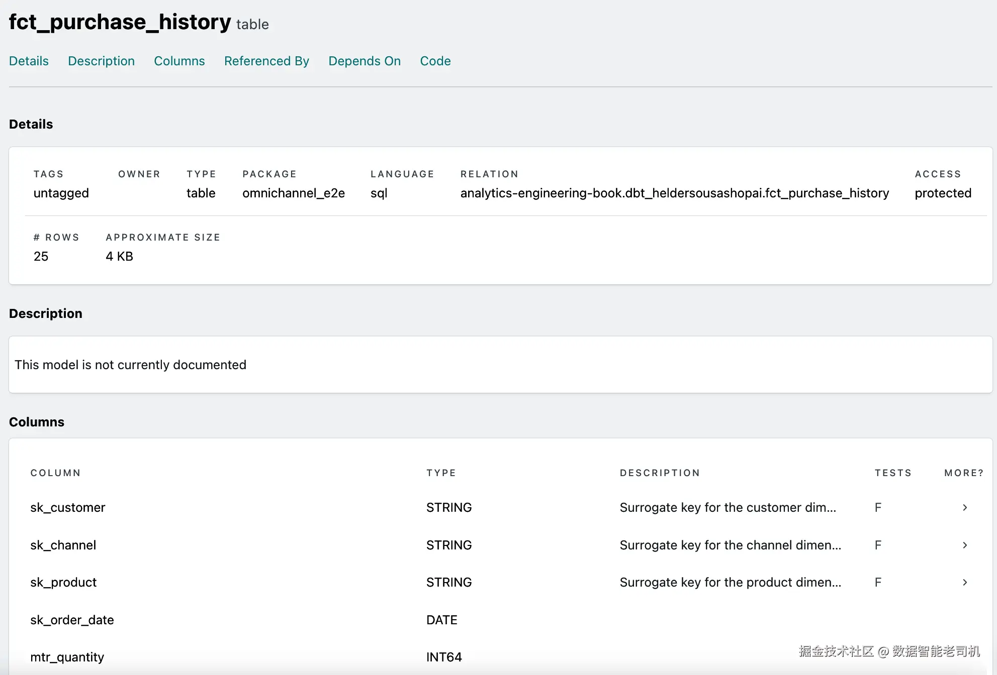
图 6-8：fct_purchase_history documentation page

就是这样。最后一步是将我们一直在做的内容部署到 production environment。为此，需要在 dbt 中创建一个 environment，类似图 6-9 所示。

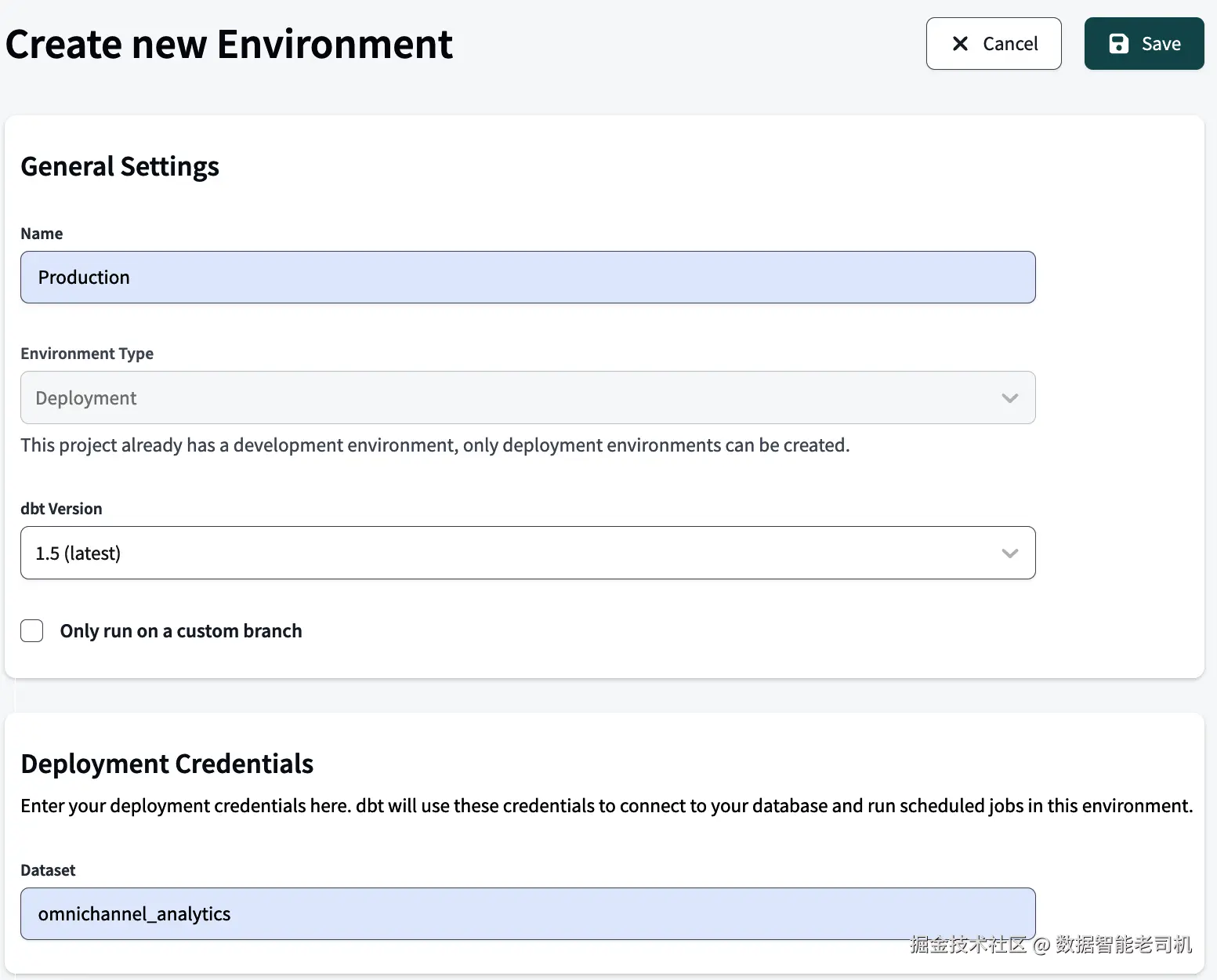
图 6-9：Creating a production environment

注意，我们将 production dataset 命名为 omnichannel_analytics。我们将在 "Data Analytics with SQL" 中使用这个 dataset。创建 environment 后，就可以配置 job。为了简洁，在 Create Job 中提供 Job name，将 environment 设置为 Production，也就是刚刚创建的 environment，勾选 "Generate docs on run"，最后在 Commands section 中，在 dbt build command 下面加入 dbt test command。其余保持默认。

Job 创建后，手动执行 job，并查看 logs。如果 logs 类似图 6-10，就是一个良好信号。

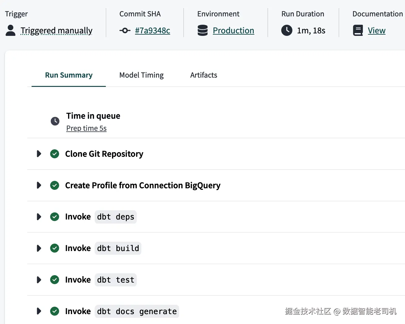
图 6-10：Job execution log

让我们查看 data platform，也就是本案例中的 BigQuery，并检查所有内容是否成功运行。BigQuery 中的 models 应该如图 6-11 所示。

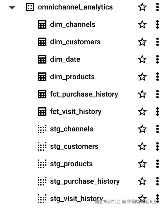
图 6-11：BigQuery 中的 models

总结来说，构建 data warehouse 的最后部分聚焦于 testing、documentation 和 go-live process。通过进行全面 tests、记录 data models，并为 production deployment 做准备，你可以确保 data warehouse 的 accuracy、reliability 和 usability。下一节中，我们将深入使用 SQL 进行 data analytics，把 data warehouse 提升到下一层级。

Data Analytics with SQL

随着 star schema model 完成，我们现在可以开始 analytics discovery phase，并开发 queries 来回答 specific business questions。如前所述，这种 data modeling technique 使我们能够轻松从 fact tables 中选择特定 metrics，并用来自 dimensions 的 attributes 对其进行 enrich。

在 Example 6-29 中，我们首先创建一个 query，用于回答 "Total amount sold per quarter with discount"。该 query 从两张 tables 中获取 data：fct_purchase_history 和 dim_date，并对检索到的数据执行 calculations。这个 query 旨在获取每个 quarter 的 total amounts 之和。

Example 6-29：Total amount sold per quarter with discount

SELECT dd.year_number,
      dd.quarter_of_year,
      ROUND(SUM(fct.mtr_total_amount_net),2) as sum_total_amount_with_discount
FROM `omnichannel_analytics`.`fct_purchase_history` fct
LEFT JOIN `omnichannel_analytics`.`dim_date` dd
                              on dd.date_day = fct.sk_order_date
GROUP BY dd.year_number,dd.quarter_of_year

通过分析运行该 query 的结果（图 6-12），可以得出结论：2023 年第二季度最好，而 2024 年第一季度最差。

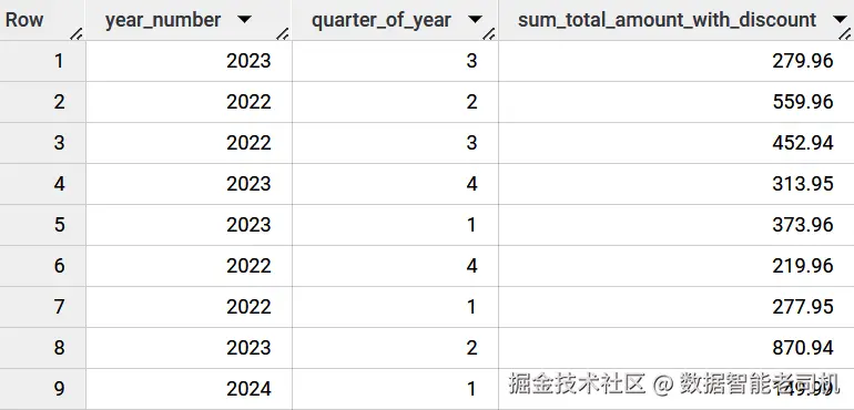
图 6-12：用于获取每季度折扣后销售总额的 analytical query

在 Example 6-30 中，我们使用 star schema model 计算每个 channel 的 average length of stay，以分钟为单位。它选择 channel name（dc.dsc_channel_name）以及 average length of stay in minutes，这个值通过 function ROUND(AVG(mtr_length_of_stay_minutes),2) 计算。dc.dsc_channel_name 指 dim_channels dimension table 中的 channel_name attribute。

ROUND(AVG(mtr_length_of_stay_minutes),2) 会对 fct_visit_history fact table 中的 mtr_length_of_stay_minutes column 使用 AVG function，计算 average length of stay in minutes。ROUND() function 用于将结果四舍五入到两位小数。Alias avg_length_of_stay_minutes 被赋给计算出的平均值。

Example 6-30：Average time spent per visit on each channel

SELECT dc.dsc_channel_name,
      ROUND(AVG(mtr_length_of_stay_minutes),2) as avg_length_of_stay_minutes
FROM `omnichannel_analytics.fct_visit_history` fct
LEFT JOIN `omnichannel_analytics.dim_channels` dc
on fct.sk_channel = dc.sk_channel
GROUP BY dc.dsc_channel_name

通过分析运行该 query 的结果（图 6-13），可以得出结论：用户在 website 上花费的时间比在 mobile app 或公司的 Instagram account 上更多。

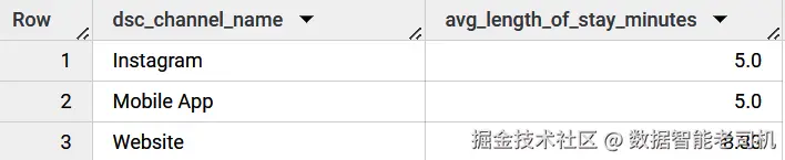
图 6-13：用于获取每个 channel 单次访问平均停留时间的 analytical query

在 Example 6-31 中，我们将 model 用于一个 advanced use case。现在我们希望获取每个 channel 的 top three products。由于我们有三个不同 channels，即 mobile app、website 和 Instagram，因此希望获得九行结果，每个 channel 各三条 best sellers。

为此，我们利用 CTEs 的结构优势，从一个 base query 开始，它会返回每个 product 和 channel 的 sum_total_amount。有了它后，可以创建第二个 CTE，从前一个 CTE 开始，按 channel 对 total amount 降序排名，也就是每个 product 在各 channels 中的 performance order。为了获得这个 rank，我们使用 window functions，具体来说是 RANK() function，它会基于前述规则为 rows 打分。

Example 6-31：Top three products per channel

WITH base_cte AS (
    SELECT dp.dsc_product_name,
           dc.dsc_channel_name,
           ROUND(SUM(fct.mtr_total_amount_net),2) as sum_total_amount
    FROM `omnichannel_analytics`.`fct_purchase_history` fct
    LEFT JOIN `omnichannel_analytics`.`dim_products` dp
                                    on dp.sk_product = fct.sk_product
    LEFT JOIN `omnichannel_analytics`.`dim_channels` dc
                                    on dc.sk_channel = fct.sk_channel
    GROUP BY dc.dsc_channel_name, dp.dsc_product_name
),
ranked_cte AS(
    SELECT base_cte.dsc_product_name,
        base_cte.dsc_channel_name,
        base_cte.sum_total_amount,
        RANK() OVER(PARTITION BY dsc_channel_name
                    ORDER BY sum_total_amount DESC) AS rank_total_amount
    FROM base_cte
)
SELECT *
FROM ranked_cte
WHERE rank_total_amount <= 3

通过分析运行该 query 的结果（图 6-14），我们得出结论：mobile app 中表现最好的产品是 Men Bomber Jacket with Detachable Hood，销售额为 €389.97；website 中表现最好的是 Leather Crossbody Handbag，销售额为 €449.97；Instagram 中表现最好的是 Unisex Running Sneakers，销售额为 €271.97。

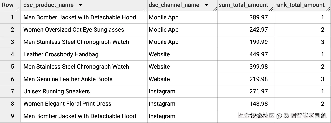
图 6-14：用于获取每个 channel top three products 的 analytical query

在 Example 6-32 中，我们通过使用刚创建的 star schema data model，对 2023 年 mobile app 上的 top customers 执行分析，从而结束这段通过 SQL 支持 business questions 的演示。我们再次利用 CTEs 正确组织 query，但这一次不是使用 window functions，而是结合 ORDER BY clause 和 LIMIT modifier，获得按 purchase 金额排序的 top three buyers。

Example 6-32：Top three customers in 2023 on the mobile app

WITH base_cte AS (
    SELECT dcu.dsc_name,
           dcu.dsc_email_address,
           dc.dsc_channel_name,
           ROUND(SUM(fct.mtr_total_amount_net),2) as sum_total_amount
    FROM `omnichannel_analytics`.`fct_purchase_history` fct
    LEFT JOIN `omnichannel_analytics`.`dim_customers` dcu
                               on dcu.sk_customer = fct.sk_customer
    LEFT JOIN `omnichannel_analytics`.`dim_channels` dc
                               on dc.sk_channel = fct.sk_channel
    WHERE dc.dsc_channel_name = 'Mobile App'
    GROUP BY dc.dsc_channel_name, dcu.dsc_name, dcu.dsc_email_address
    ORDER BY sum_total_amount DESC
)
SELECT *
FROM base_cte
LIMIT 3

通过分析运行该 query 的结果（图 6-15），可以得出结论：top buyer 是 Sophia Garcia，她消费了 €389.97。我们可以给她发送 email 到 sophia.garcia@emailaddress.com，感谢她作为如此特别的 customer。

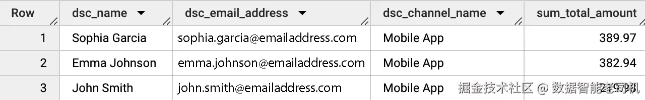
图 6-15：用于获取 mobile app top customers 的 analytical query

通过展示这些 queries，我们希望强调使用 star schema 回答 complex business questions 的内在 simplicity 和 effectiveness。借助这种 schema design，组织可以更高效地获得 valuable insights，并做出 data-driven decisions。

虽然前面的 queries 展示了每个 query 的简洁性，但真正的力量在于能够将它们与 CTEs 结合起来。这种 strategic use of CTEs 使 queries 能够以结构化且易理解的方式优化和组织。通过使用 CTEs，analysts 可以 streamline workflows，提升 code readability，并促进 intermediate results 的复用。

此外，使用 window functions 会为 data analysis 增加额外的效率层。借助 window functions，analysts 可以在特定 data partitions 或 windows 上高效计算 aggregated results，为 trends、rankings 和 comparative analyses 提供 valuable insights。通过使用这些 functions，analysts 可以从 large datasets 中高效推导 meaningful conclusions，加速 decision-making process。

写作本节的目的，是概括本书所覆盖主题的重要意义。它强调了扎实掌握 SQL、熟练的数据建模能力，以及全面理解围绕 dbt 等数据技术的技术格局，对于提升 analytics engineering skills 的重要性。获得这些能力，使 professionals 能够有效驾驭企业或个人项目中生成的海量 data。

Conclusion

Analytics engineering 的格局如人类想象力的边界一样广阔且多样。就像 Tony Stark 利用 cutting-edge technology 转变为 Iron Man 一样，我们也被 databases、SQL 和 dbt 赋能，使我们不只是 data-driven age 的旁观者，而是主动参与其中的 heroes。就像 Stark 的各种 armor，这些工具为我们提供 flexibility、strength 和 precision，使我们能够正面应对最复杂的 challenges。

Databases 和 SQL 一直是 data-driven strategies 的 foundational pillars，提供 stability 和 reliability。然而，随着 demands 和 complexities 增长，analytics 已经扩展到集成复杂 data modeling practices。这种转变不只是 mechanics 层面的变化，它更强调 crafting business narratives、anticipating analytical trends，以及为 future requirements 进行 forward planning。

dbt 已经成为这个动态格局中的 transformational element。它不只是 SQL 的补充，更重新定义了我们处理 collaboration、testing 和 documentation 的方式。借助 dbt，raw 和 fragmented data 的处理变得更加 refined，最终形成支持 informed decision making 的 actionable models。

Analytical engineering 融合了 traditional practices 和 innovative advancements。虽然 data modeling、rigorous testing 和 transparent documentation 有既定原则，但 dbt 这样的工具引入了新的方法和可能性。每个面对的 challenge，无论是对刚进入这个领域的人，还是对有经验的人来说，都是一次学习机会。每个 database 和 query 都提供一种独特视角和一种潜在 solution。

就像 Holmes 能从 fragmentary evidence 中编织出 labyrinthine stories，analytics engineers 也能从高度 fragmented data points 中创建 compelling data models。他们手中的工具不只是 mechanical，而是赋能他们 anticipate analytic trends、align data models with business needs，并像 Holmes 一样成为 data-driven age 的 storytellers。在这个 context 中，dbt 就是他们的 Watson，促进 collaboration 和 efficiency，就像这位著名侦探值得信赖的同伴。与 Holmes 的相似之处非常鲜明：二者都把揭示隐藏在 cryptic cases 或 complex datasets 中的秘密作为使命。我们希望通过本书各章，你已经获得 insights，并对这门不断演进的学科有了更清晰的理解。