《遗传算法：从自然选择到Rastrigin函数优化，手写一个完整的进化求解器》

摘要

遗传算法 GA（Genetic Algorithm） 是一种通过模拟自然界遗传和进化机制的随机化搜索方法，将方法解编码为自然界个体，通过选择、交叉和变异 操作，在群体中迭代进化出最优个体。本文将从编码策略、算子设计系统介绍 GA 的数学机理，并以寻找 Rastrigin 多峰函数最值问题为例手写算法实现。

引言

在面对复杂非线性优化问题时使用常规通用的计算方法往往无法解决问题，如

非线性问题则无法通过求梯度寻找最优值位置。
多峰函数问题容易陷入局部最优。
目标函数不可导时无法通过求导计算最优值。

优化算法的出现很好的解决这类问题，如遗传算法 GA通过模拟自然进化解决：

群体搜索：传统算法只针对一个解进行优化，而遗传算法通过多个解并行优化
适应度函数：遗传算法只需要知道一个解的好坏（适应度函数值），不需要求导和梯度
交叉算子：交叉算法实现将两个优秀的解随机片段拼接，产生一个新的解
变异算子：避免所有的解陷入局部最优，变异随机修改解的片段有助于跳出局部最优

核心原理

遗传算法的核心在于对自然界的模拟，将现实中的问题转化为自然界的问题，《Adaptation in Natural and Artificial Systems》是 John H. Holland 于 1975 年出版的里程碑式著作。这本书不仅是遗传算法（GA）的奠基之作，更提出了一套跨学科的通用适应理论。

提出的适应的基本三要素有：

结构 (Structures)： 受环境影响并被修改的对象，如遗传学中的染色体。
性能(Performance)： 衡量结构在特定环境下表现的准则，即"适应度" 。
算子 (Operators)： 应用于结构以产生新结构的手段，如交叉和变异。

整体的执行流程就是：将现实问题编码为自然界问题（结构），编写衡量问题解好坏的准则（性能），结合当前问题解产生新的解（算子），整体原理如下：

编码

核心原理：将现实问题中的"解"转化为GA可以操作的"染色体"。

二进制编码：

现实问题解的空间往往是连续的，很难从无限的空间中寻找最优解，二进制编码模拟生物染色体结构，将问题的实数解区间映射到二进制表达的区间内。

二进制位数 n ：n 位二进制数可表示的范围 <math xmlns="http://www.w3.org/1998/Math/MathML"> [ 0 , 2 n − 1 ] [0,2^n-1] </math>[0,2n−1]
精度 p ：如果仅考虑将实数区间 <math xmlns="http://www.w3.org/1998/Math/MathML"> [ L , R ] [L,R] </math>[L,R] 的整数转为二进制，精度则是 1 ，但是精度太高无法精准计算最优解，往往使用更小的 0.01 和 0.001，计算公式为： <math xmlns="http://www.w3.org/1998/Math/MathML"> p = R − L 2 n − 1 p = \frac{R-L}{2^n-1} </math>p=2n−1R−L。
编码：将实数区间 <math xmlns="http://www.w3.org/1998/Math/MathML"> [ L , R ] [L,R] </math>[L,R] 实数 x 转化为二进制编码公式

<math xmlns="http://www.w3.org/1998/Math/MathML" display="block"> D = r o u n d ( x − L R − L ∗ ( 2 n − 1 ) ) D = round \Big(\frac{x-L}{R-L} * (2^n-1) \Big ) </math>D=round(R−Lx−L∗(2n−1))

计算得到的 D 就是新区间 <math xmlns="http://www.w3.org/1998/Math/MathML"> [ 0 , 2 n − 1 ] [0,2^n-1] </math>[0,2n−1] 中的实数，再计算二进制就是 GA 操作的染色体。

<math xmlns="http://www.w3.org/1998/Math/MathML"> x − L R − L \frac{x-L}{R-L} </math>R−Lx−L 的作用是归一化 ，计算 x 在区间 <math xmlns="http://www.w3.org/1998/Math/MathML"> [ L , R ] [L,R] </math>[L,R] 内的位置， <math xmlns="http://www.w3.org/1998/Math/MathML"> ( x − L R − L ) ∗ 2 n − 1 (\frac{x-L}{R-L}) * 2^n-1 </math>(R−Lx−L)∗2n−1 归一化后再乘 <math xmlns="http://www.w3.org/1998/Math/MathML"> 2 n − 1 2^n-1 </math>2n−1 作用就是投影到新区间内。

假设我的实数区间为 <math xmlns="http://www.w3.org/1998/Math/MathML"> [ 0 , 5 ] [0,5] </math>[0,5]，使用 <math xmlns="http://www.w3.org/1998/Math/MathML"> n = 4 n=4 </math>n=4 二进制数表达：

表达范围： <math xmlns="http://www.w3.org/1998/Math/MathML"> [ 0 , 2 4 − 1 ] [0,2^4-1] </math>[0,24−1]就是 0-15
精度： <math xmlns="http://www.w3.org/1998/Math/MathML"> p = R − L 2 n − 1 = 5 15 = 0.3333 p = \frac{R-L}{2^n-1} = \frac{5}{15} = 0.3333 </math>p=2n−1R−L=155=0.3333，简单理解就是只存在 p 的倍数，即[0,0.3333] 表示的是0，因为精度有限。
编码：取 <math xmlns="http://www.w3.org/1998/Math/MathML"> x = 2 x = 2 </math>x=2 编码，归一化 <math xmlns="http://www.w3.org/1998/Math/MathML"> x − L R − L = 2 5 \frac{x-L}{R-L} = \frac{2}{5} </math>R−Lx−L=52，投影 <math xmlns="http://www.w3.org/1998/Math/MathML"> ( x − L R − L ) ∗ 2 n − 1 = 2 5 ∗ 15 = 6 (\frac{x-L}{R-L}) * 2^n-1 = \frac{2}{5} * 15 = 6 </math>(R−Lx−L)∗2n−1=52∗15=6，再计算二进制 0110，这个就是GA使用的编码。

实数编码

二进制编码如果想提高精度，就需要增加二进制长度，会导致搜索空间呈指数级增长，增加计算负担 。而实数编码是直接使用浮点数如（1.23456789）作为基因位。

精度取决于计算机中浮点数的表示精度 ，如在 Python 或 C++（double 类型）中，实数编码可以提供约 15 到 17 位有效数字的精度。

适应度函数

衡量染色体"好坏"的标准。GA 只要求能计算适应度，不要求可导。

非负：适应度必须非负，因为后续选择阶段需要用来计算
最大值问题：可直接使用目标函数作为适应度函数 <math xmlns="http://www.w3.org/1998/Math/MathML"> f i t n e s s = f ( x ) fitness=f(x) </math>fitness=f(x)
最小值问题 : 可使用最大值减法 <math xmlns="http://www.w3.org/1998/Math/MathML"> f i t n e s s = C m a x − f ( x ) fitness=C_{max} - f(x) </math>fitness=Cmax−f(x) 或取倒数

选择

经过一轮迭代，可以知道种群内所有个体的适应度大小（取最大值为例），根据达尔文进化论的"优胜劣汰"准则，应该保留适应度更大的进入下一代。

设种群 <math xmlns="http://www.w3.org/1998/Math/MathML"> N = 100 N = 100 </math>N=100 ，个体 <math xmlns="http://www.w3.org/1998/Math/MathML"> ( x 1 , x 2 , ... ... , x 100 ) (x_1,x_2,......,x_{100}) </math>(x1,x2,......,x100) ，适应度 <math xmlns="http://www.w3.org/1998/Math/MathML"> ( f 1 , f 2 , ... ... , f 100 ) (f_1,f_2,......,f_{100}) </math>(f1,f2,......,f100)

轮盘赌

按照个体的适应度大小作为被选择的概率根据，求最大值问题中，适应度越大，概率则越大
<math xmlns="http://www.w3.org/1998/Math/MathML" display="block"> p ( x i ) = f i ∑ j = 1 N f j p(x_i) = \frac{f_i}{\sum_{j=1}^{N}f_j} </math>p(xi)=∑j=1Nfjfi

优点：计算简单
缺点：当适应度差异大时，低适应度个体几乎没有机会

锦标赛

随机选 k 个个体（通常 k=3），其中适应度最高者胜出

优点：不依赖全局适应度总和，并行友好
缺点：k 太大会过早收敛

精英保留

直接保留当代中适应度最高的 1 - 2 个个体直接复制到下一代，且不参与后面的交叉与变异。

优点：避免适应度高个体被淘汰，防止最优解被交叉变异破坏
缺点：可能陷入局部最优

交叉

模拟"基因重组"，将两个父代的好基因片段组合产生新个体。

二进制编码交叉

单点交叉：随机选一个交叉点，交换两侧基因
两点交叉：随机选两个点，交换中间片段
均匀交叉：每个基因位独立以 0.5 概率交换

实数编码交叉

算术交叉：

<math xmlns="http://www.w3.org/1998/Math/MathML" display="block"> x c h i l d = α ∗ x p 1 + ( 1 − α ) ∗ x p 2 , α ∈ [ 0 , 1 ] x_{child} = \alpha *x_{p1}+(1-\alpha)*x_{p2},\alpha∈[0,1] </math>xchild=α∗xp1+(1−α)∗xp2,α∈[0,1]

并不是所有的个体都要交叉，会设置交叉概率 <math xmlns="http://www.w3.org/1998/Math/MathML"> P c P_c </math>Pc ，通常取 <math xmlns="http://www.w3.org/1998/Math/MathML"> [ 0.5 , 0.9 ] [0.5,0.9] </math>[0.5,0.9]，

<math xmlns="http://www.w3.org/1998/Math/MathML"> P c P_c </math>Pc 过大 → 种群动荡， <math xmlns="http://www.w3.org/1998/Math/MathML"> P c P_c </math>Pc 过小 → 搜索停滞。

变异

模拟"基因突变"，随机扰动基因值以维持种群多样性，防止早熟收敛。

重点内容：

二进制变异 ：每个基因位以 <math xmlns="http://www.w3.org/1998/Math/MathML"> P m P_m </math>Pm 概率翻转（0→1，1→0）
实数变异 ：高斯变异 <math xmlns="http://www.w3.org/1998/Math/MathML"> x n e w = x o l d + N ( 0 , σ 2 ) x_{new}=x_{old}+N(0,σ^2) </math>xnew=xold+N(0,σ2)
变异概率 <math xmlns="http://www.w3.org/1998/Math/MathML"> P m P_m </math>Pm：通常很小（0.001-0.1），过大 → 退化为随机搜索，过小 → 多样性不足
与交叉的分工：交叉负责全局搜索（探索），变异负责局部微调（开发）

算法流程

1.全局参数初始化

种群数量 ：现实问题中解的数量，种群中个体的数量
基因长度 ：二进制编码位数
迭代次数 ：迭代的轮次数量
交叉概率 ：个体基因和其他个体发生交叉的概率
变异概率 ：个体基因发生变异的概率

2.基因解码

初始化种群个体数据是编码后的，适应度函数参数是现实问题实数区间的。

计算的公式就是编码公式的变式：
<math xmlns="http://www.w3.org/1998/Math/MathML" display="block"> x = D ∗ ( R − L ) 2 n − 1 + L x=\frac{D * (R-L)}{2^n-1 } + L </math>x=2n−1D∗(R−L)+L

二进制转十进制：将个体基因从二进制转为十进制数 D
归一化：计算该数据在个体数据中的位置 <math xmlns="http://www.w3.org/1998/Math/MathML"> D 2 n − 1 \frac{D}{2^n-1 } </math>2n−1D
投影： <math xmlns="http://www.w3.org/1998/Math/MathML"> D 2 n − 1 ( R − L ) \frac{D}{2^n-1 }(R-L) </math>2n−1D(R−L)，映射到实际区间中
偏移： <math xmlns="http://www.w3.org/1998/Math/MathML"> D 2 n − 1 ( R − L ) + L \frac{D}{2^n-1 }(R-L) + L </math>2n−1D(R−L)+L，数据偏移以 L 为起点

3.计算适应值

遗传算法通常的适应值不能为负数，避免出现负数可进行下面处理

当前值 - 本轮最小值得到的结果一定大于等于0
为了避免等于0情况，可额外添加一个极小值如 1e-3

4.选择

选择更优秀的个体基因保留用于后续的交叉和变异：

轮盘赌 ：每个个体的概率如 <math xmlns="http://www.w3.org/1998/Math/MathML"> p = f f . s u m ( ) p=\frac{f}{f.sum()} </math>p=f.sum()f ，可看作一个圆盘 p 就是该个体的占比
锦标赛 ：从种群中随机选择 k 个，进行 N（种群数量）轮，每轮选择适应度最高的
精英保留 ：不是完整的选择算法，基于上面的选择手动保留精英个体，剩下的依旧进行选择

5.交叉变异

选择完优秀个体后，就会对个体概率进行交叉和变异，每个个体都有 <math xmlns="http://www.w3.org/1998/Math/MathML"> P c P_c </math>Pc 发生交叉，随机选择另一个解和交叉位置每个都有 <math xmlns="http://www.w3.org/1998/Math/MathML"> P m P_m </math>Pm 发生变异，随机选择变异位置基因取反。

交叉：遍历到个体1时，随机生成一个 0-1 的随机数，如果小于 <math xmlns="http://www.w3.org/1998/Math/MathML"> P c P_c </math>Pc 则交叉，个体2随机选择，交叉发生的位置也随机选择，取个体1和个体2的上下部分结合形成两个新个体，加入后代种群。
变异：模拟"基因突变"，每个个体有概率 <math xmlns="http://www.w3.org/1998/Math/MathML"> P m P_m </math>Pm 发生变异，变异位置随机。

手写 GA

根据上面的算法实现遗传算法mvp 。

染色体：二进制串，长度 = dna_size × dim
选择：轮盘赌
交叉：单点交叉（二进制）
变异：位翻转

python 复制代码

import numpy as np


class MyGA:
    """ mini 遗传算法类
    """

    def __init__(self, pop_size=100, dna_size=10, n_generation=100, cross_rate=0.8, mutation_rate=0.01, dim=None):
        """ 初始化
        """
        self.pop_size = pop_size  # 种群数量
        self.dna_size = dna_size  # 基因长度
        self.n_generation = n_generation  # 迭代次数
        self.cross_rate = cross_rate  # 交叉概率
        self.mutation_rate = mutation_rate  # 变异概率
        self.dim = dim  # 维度

    def _translate_dna(self, pop, limit):
        """解码
            将编码后的二进制数据转换回原本实际区间数据
            遵循公式 ： x = [D·(R-L)/(2^n - 1)]+L
        """
        # 1.二进制-->十进制
        pop_reshaped = pop.reshape(self.pop_size, self.dim, self.dna_size)
        powers = 2 ** np.arange(self.dna_size - 1, -1, -1)
        decimal_values = np.dot(pop_reshaped, powers)
        # 2.归一化
        max_decimal = 2 ** self.dna_size - 1
        normalized = decimal_values / max_decimal
        # 3.映射到实际区间[L,R]
        L = limit[:, 0]
        R = limit[:, 1]
        decoded = normalized * (R - L) + L
        return decoded

    def _get_fitness(self, fitness_function, x):
        """计算适应值
            不允许存在负数，若存在负数，考虑整体上移
        """
        # 求最大值
        pred = fitness_function(x)
        return pred - np.min(pred) + 1e-3
        # 求最小值
        # return np.max(pred)-pred + 1e-3

    def _select(self, fitness, pop):
        """选择（轮盘赌）
            按照概率选择保留的解
        """
        idx = np.random.choice(np.arange(self.pop_size), size=self.pop_size,
                               replace=True, p=fitness / fitness.sum())
        return pop[idx]

    def _evolve(self, pop):
        """交叉变异
            每个解都有 cross_rate 发生交叉，随机选择另一个解和交叉位置
            每个都有 mutation_rate 发生变异，随机选择变异位置基因取反
        """
        new_pop = []
        for father in pop:
            # 交叉
            child = father.copy()
            if np.random.rand() < self.cross_rate:
                mother = pop[np.random.randint(self.pop_size)]
                cross_point = np.random.randint(0, self.dna_size * self.dim)
                child[cross_point:] = mother[cross_point:]
            # 变异
            if np.random.rand() < self.mutation_rate:
                mutate_point = np.random.randint(0, self.dna_size * self.dim)
                child[mutate_point] ^= 1
            new_pop.append(child)
        return np.array(new_pop)

    def optimize(self, fitness_function, limit):
        """ 算法实现
        """
        # 1.参数初始化
        # np.random.seed(42)
        pop = np.random.randint(2, size=(self.pop_size, self.dna_size * self.dim))
        # 2.迭代计算
        for i in range(self.n_generation):
            # 3.DNA解码
            x = self._translate_dna(pop, limit)
            # 4.计算适应值
            fitness = self._get_fitness(fitness_function, x)
            # 5.轮盘赌
            pop = self._select(fitness, pop)
            # 6.交叉变异
            pop = self._evolve(pop)
        # 7.寻找最优解
        final_x = self._translate_dna(pop, limit)
        final_fit = fitness_function(final_x)
        return final_x[np.argmax(final_fit)]

使用手写GA 计算二维的 Rastrigin函数最大值，已知最大值点在[+-4.5,+-4.5]，最大值大概为 80

python 复制代码

def FitnessFunction(x):
    """Rastrigin适应度函数
    """
    n = x.shape[1]
    return 10 * n + np.sum(x ** 2 - 10 * np.cos(2 * np.pi * x), axis=1)


if __name__ == '__main__':
    # 维度为2测试结果
    ga = MyGA(dim=2)
    limits = np.array([[-5.12, 5.12], [-5.12, 5.12]])
    ga_optimize = ga.optimize(FitnessFunction, limits)
    print(f"最终找到的最优解坐标: {ga_optimize}")
    print(f"对应的函数最大值: {FitnessFunction(ga_optimize.reshape(1, -1))[0]}")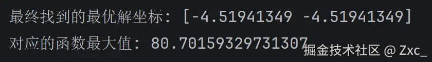

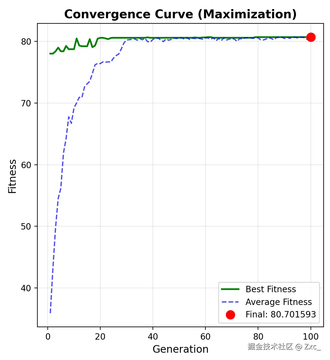
求最大值的适应度变化曲线：

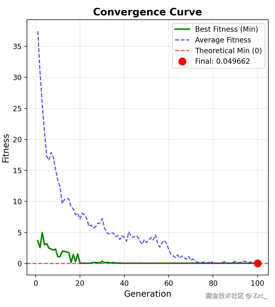
求最小值的适应度变化曲线：

画图函数需要的可以到Optimization/GS at main · Study944/Optimization

DEAP库

Deap实现是通过自主搭建算法执行流程，如搭建积木（算子）一般，其核心概念有四个：

creator(创建者)：用于动态创建新的类
toolbox(工具箱)：用于定于算法操作如（如何生成个体，如何交叉和变异等）
algorithms(内建算法)：提供一些写好的算法流程
tools(算子库)：提供一些写好的遗传操作如（轮盘赌和单点交叉）

python 复制代码

import random
import numpy as np
from deap import base, creator, tools, algorithms

# 1. 定义问题：最大化适应度
creator.create("FitnessMax", base.Fitness, weights=(1.0,))
creator.create("Individual", list, fitness=creator.FitnessMax)

# 参数设置
DIM = 2  # 维度
DNA_SIZE = 20  # 每个维度的二进制位数
POP_SIZE = 100  # 种群数量
N_GEN = 100  # 迭代次数
LIMIT = [-5.12, 5.12]  # 变量范围

toolbox = base.Toolbox()

# 2. 编码实现：注册二进制基因生成器
toolbox.register("attr_bin", random.randint, 0, 1)
# 个体由 DIM * DNA_SIZE 个二进制位组成
toolbox.register("individual", tools.initRepeat, creator.Individual,
                 toolbox.attr_bin, n=DNA_SIZE * DIM)
toolbox.register("population", tools.initRepeat, list, toolbox.individual)


def decode(individual):
    """解码逻辑：将二进制个体映射回连续空间的实数向量"""
    x = []
    max_decimal = 2 ** DNA_SIZE - 1
    for i in range(DIM):
        # 截取对应维度的基因段
        start = i * DNA_SIZE
        end = (i + 1) * DNA_SIZE
        gene_segment = individual[start:end]
        # 二进制转十进制
        decimal_d = 0
        for bit in gene_segment:
            decimal_d = (decimal_d << 1) | bit
        # 映射公式：L + (D / (2^n - 1)) * (R - L)
        res = LIMIT[0] + (decimal_d / max_decimal) * (LIMIT[1] - LIMIT[0])
        x.append(res)
    return np.array(x)


def evalRastrigin(individual):
    """适应度评估：包含解码过程"""
    x = decode(individual)
    n = len(x)
    # 计算Rastrigin函数值（原本连续空间的数据）
    fitness_value = 10 * n + np.sum(x ** 2 - 10 * np.cos(2 * np.pi * x))
    return (fitness_value,)


# 3. 注册遗传算子
toolbox.register("evaluate", evalRastrigin)
toolbox.register("mate", tools.cxTwoPoint)  # 二进制常用两点交叉
toolbox.register("mutate", tools.mutFlipBit, indpb=0.01)  # 二进制位翻转变异
# toolbox.register("select", tools.selRoulette)   # 轮盘赌
toolbox.register("select", tools.selTournament, tournsize=3)  # 锦标赛选择


def main():
    # 初始化种群
    population = toolbox.population(n=POP_SIZE)

    # 精英保留：HallOfFame 自动保留历史最优个体
    hof = tools.HallOfFame(1)

    # 统计插件
    stats = tools.Statistics(lambda ind: ind.fitness.values)
    stats.register("avg", np.mean)
    stats.register("min", np.min)
    stats.register("max", np.max)

    # 4. 运行进化算法（eaSimple）
    pop, log = algorithms.eaSimple(population, toolbox,
                                   cxpb=0.8,  # 对应 cross_rate
                                   mutpb=0.1,  # 个体变异概率
                                   ngen=N_GEN,
                                   stats=stats,
                                   halloffame=hof,
                                   verbose=True)

    # 输出结果
    best_ind = hof[0]
    best_x = decode(best_ind)
    print("-" * 30)
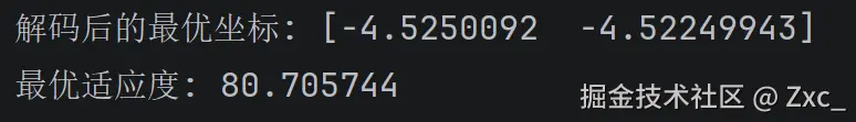
    print(f"最优解编码: {best_ind}")
    print(f"解码后的最优坐标: {best_x}")
    print(f"最优适应度: {best_ind.fitness.values[0]:.6f}")

    return pop, log, hof


if __name__ == "__main__":
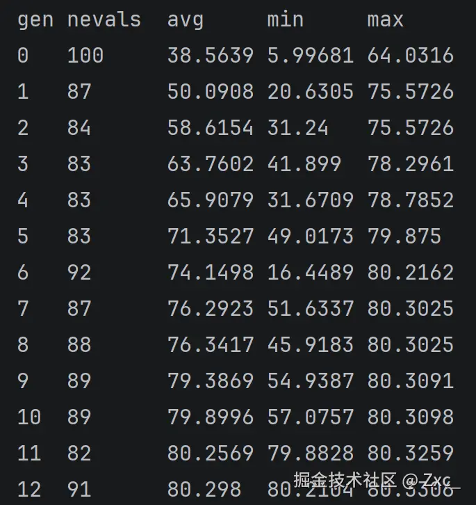
    main()

Deap 默认开启记录每轮的核心参数，平均适应度和最小最大适应度，大概在10轮前后就能稳定。

参数实验

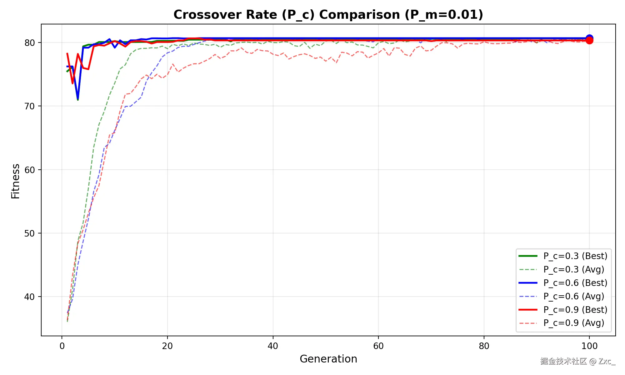
测试在不同的交叉概率下 GA 函数寻找最优值的效果：

<math xmlns="http://www.w3.org/1998/Math/MathML"> p m = 0.01 , p c = [ 0.3 , 0.6 , 0.9 ] p_m = 0.01 ,p_c=[0.3,0.6,0.9] </math>pm=0.01,pc=[0.3,0.6,0.9]

Pc = 0.3时收敛缓慢，因为优秀基因片段无法充分重组；Pc = 0.9时虽初期收敛最快，但后期震荡明显，因为高交叉率破坏了已形成的优秀解结构；Pc = 0.8在收敛速度和稳定性之间达到较好平衡。

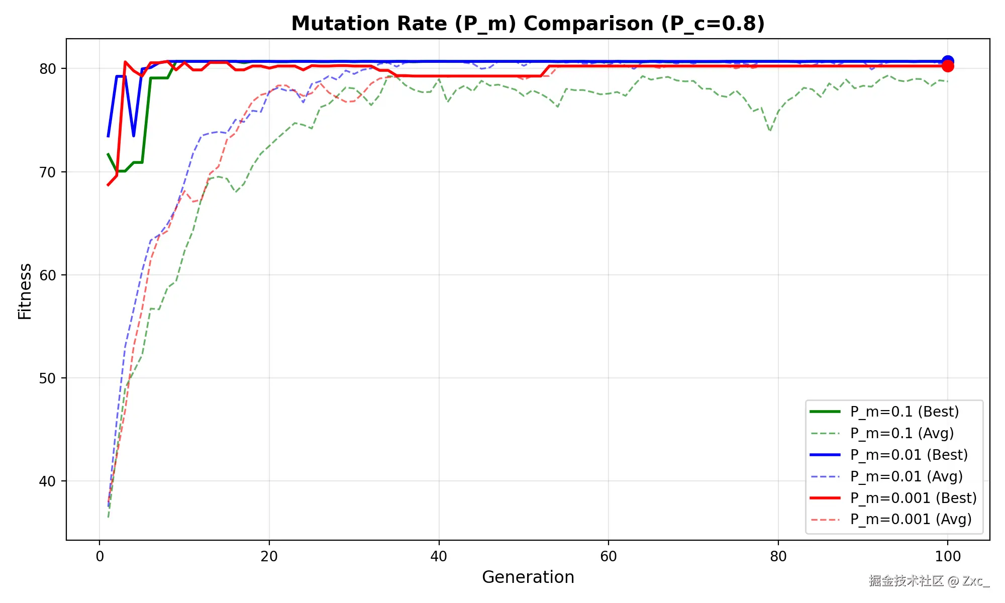
<math xmlns="http://www.w3.org/1998/Math/MathML"> p c = 0.8 , p m = [ 0.1 , 0.01 , 0.001 ] p_c = 0.8 ,p_m=[0.1,0.01,0.001] </math>pc=0.8,pm=[0.1,0.01,0.001]

Pm = 0.1时曲线全程震荡，几乎退化为随机搜索；Pm = 0.001时收敛过慢，种群多样性不足；Pm = 0.01在保持搜索方向的同时提供了足够的局部探索能力。

前沿进展

自适应 GA ： <math xmlns="http://www.w3.org/1998/Math/MathML"> P c P_c </math>Pc 和 <math xmlns="http://www.w3.org/1998/Math/MathML"> P m P_m </math>Pm 随种群多样性自动调整。当种群多样性高时减小交叉/变异压力，低时增大
多目标 GA（NSGA-II） ：非支配排序 + 拥挤度距离。与 PSO 文章中的 MOPSO 形成"多目标优化双雄"呼应
并行 GA：岛屿模型（各子种群独立进化，定期迁移个体）。个体适应度评估天然独立，直接对接"网络与并行计算"
GA 在机器学习中的应用：KNN 的 K 值选择、线性回归的 λ 整定，GA 都可替代网格搜索和 PSO

总结

GA 和 PSO 对比图

维度	GA	PSO
搜索机制	自然选择 + 基因重组	个体记忆 + 社会分享
编码方式	二进制/实数/排列	实数向量
收敛速度	较慢	较快
适用场景	组合优化、特征选择	连续函数优化

代码开源：Optimization/GA at main · Study944/Optimization

参考文献

Holland J H. Adaptation in Natural and Artificial Systems. MIT Press, 1975.
Goldberg D E. Genetic Algorithms in Search, Optimization and Machine Learning. Addison-Wesley, 1989.
Deb K, et al. A fast and elitist multiobjective genetic algorithm: NSGA-II. IEEE TEC, 2002.
Rudolph G. Convergence analysis of canonical genetic algorithms. IEEE TNN, 1994.